9. Regression analysis
Since version 0.15, we have also the ability to perform a regression analysis at the drug level (ODAF mode).
The are currently 3 types of regression implemented:
- Ridge
- Lasso
- Elastic Net
Information about functionalities implemented in GDSCTools are available
in the reference gdsctools.regression. and in a notebook (see https://github.com/CancerRxGene/gdsctools/tree/master/notebooks) called Regression.
We first give some examples following information contained in the reference and the notebook. In the example here below, the data sets are small. In practice, you may have many features and would require a cluster to perform the computation in a reasonable amount of time. We therefore develop a pipeline that wraps up the analysis. The pipeline uses the Snakemake framework (see below).
Warning
you must install Snakemake, in which case you must use Python >=3.5
9.1. Doing the analysis using GDSCTools library
As usual, we will use some data provided in GDSCTools in the form of ain IC50 data set and a genomic features data set:
from gdsctools import *
ic50 = IC50(ic50_v17)
gf = GenomicFeatures(gf_v17)
To decrease the computational time, let us select only genomic features that are factors or mutations:
gf.df = gf.df[[x for x in gf.df.columns if "FACTOR" in x or "mut" in x]]
Here, we will use the Lasso regression:
lasso = GDSCLasso(ic50, gf)
For each drug, all features are taken and a regression is performed. For each drug, we tune the alpha parameter using a cross validation (a K-fold CV).
Note
the regression implementation is based on scikit-learn. The alpha parameter is called lambda in the R glmnet package. In the ElasticNet case, and additional parameter is called l1_ratio (0.5 by default) and corresponds to the glmnet parameter alpha.
Before, doing the tuning, let us choose one drug. Let us pick up an interesting one:
drugid = 1047
9.1.1. Tuning
Users are able to choose the number of K-folds, which is set to 10 by default. Here is the method to call:
res = lasso.runCV(drugid, kfolds=8)
The returned object contains the best alpha but also the pearson coefficient:
res.alpha
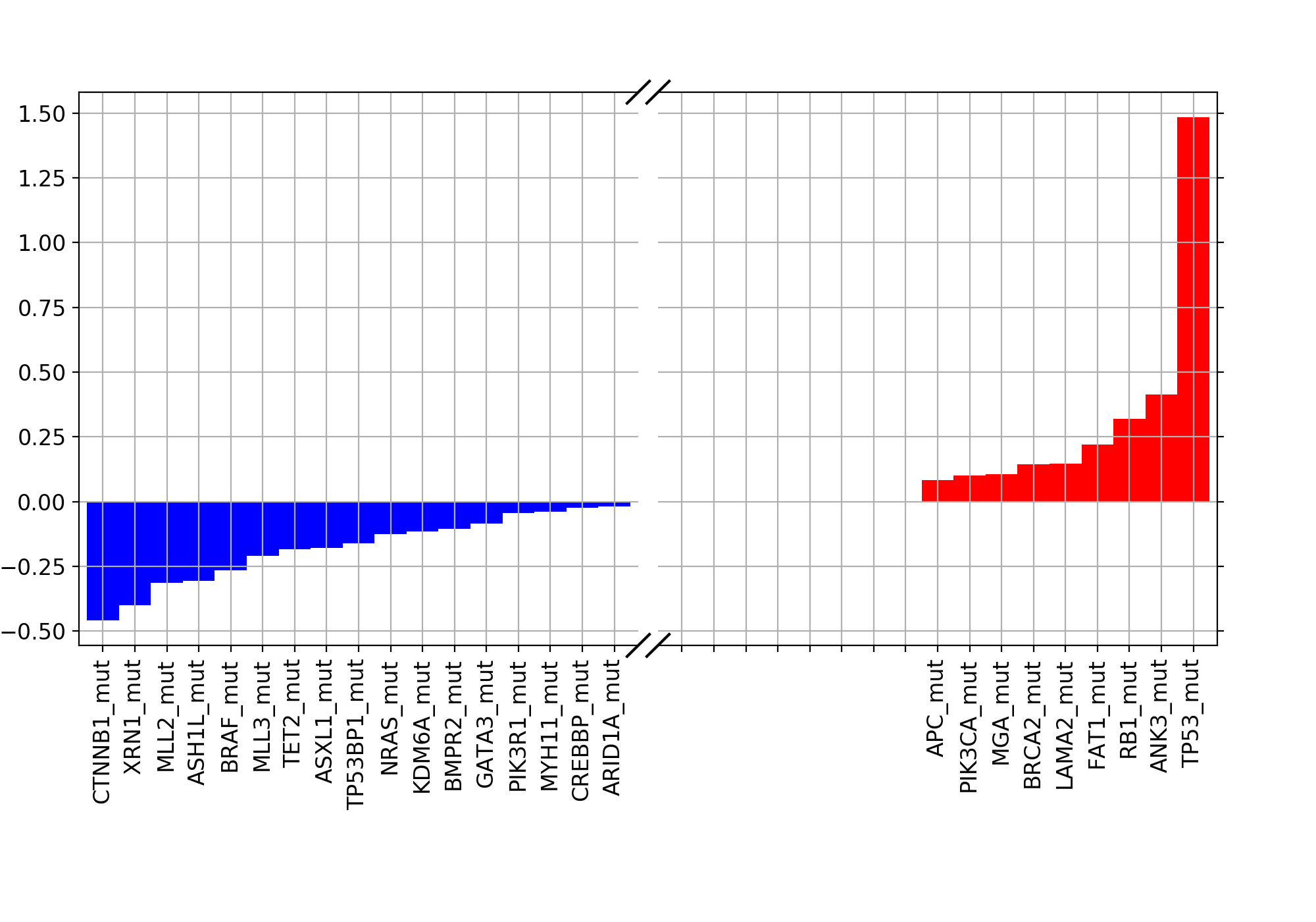
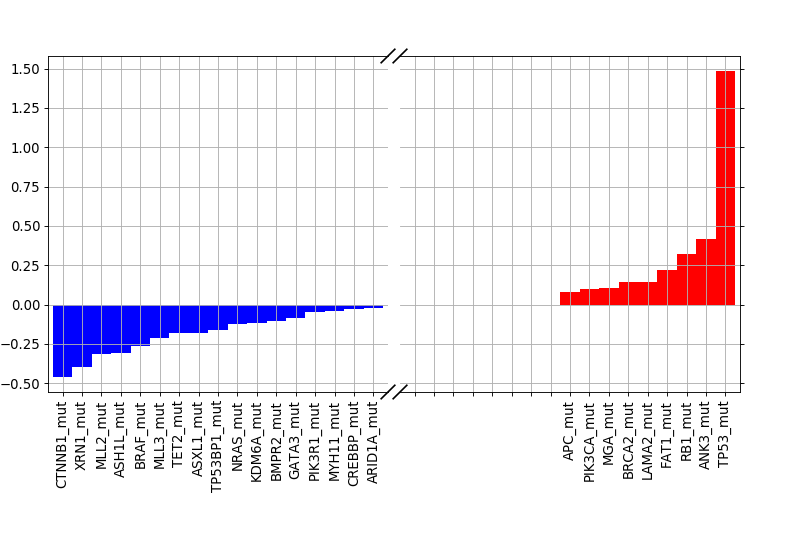
From this parameter, the best model can be created and used for further analysis, in particular to see the important features:
best_model = lasso.get_model(alpha=res.alpha)
weights = lasso.plot_weight(drugid, best_model)
(Source code, png, hires.png, pdf)
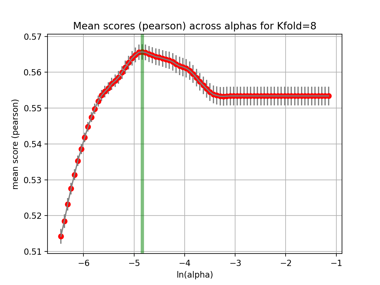
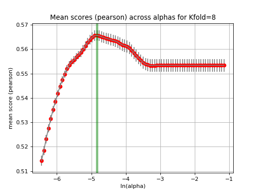
9.1.2. Validation
The runCV function mentionned above does not plot any figures for optimisation reasons. We implemented another function called tune_alpha, which has a visual representation. This is however 20 time slower than runCV and is not used in production.:
lasso.tune_alpha(drugid, alpha_range=[-2.8,-0.5])
(Source code, png, hires.png, pdf)
Another important function is the check_randomness method. It runs N times
the gdsctools.regression.GDSCLAsso.runCV() function, and N times the
same analysis shuffling the Y
data. This creates a NULL model. The Pearson correlation values between the NULL
model and the real data is then compared using a Bayes factor metric
(independent of N).
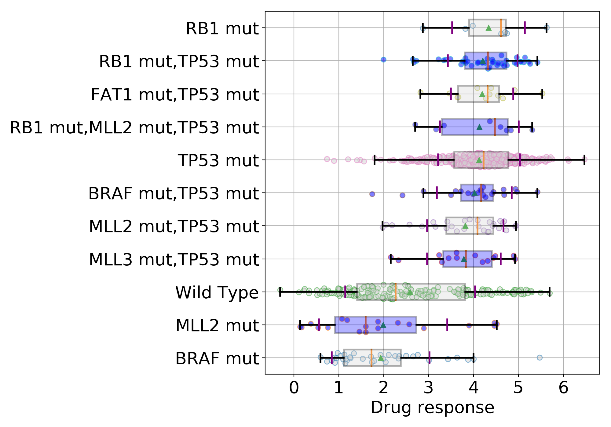
9.1.3. boxplots
boxplots = lasso.boxplot(drugid, model=best_model, n=10, bx_vert=False)
(Source code, png, hires.png, pdf)

9.1.4. ADAF analysis
We have now a good picture of what the regression tools can do. If one wants to play with ElasticNet or Ridge methods, just replaced GDSCLasso by GDSCElasticNet or GDSCRidge.
We now want to run the regression on all drugs. This can be done manually of course using a loop over each drug identifiers:
for drugID in lasso.drugIds:
    res = lasso.runCV(drugid, kfolds=8)
    best_model = lasso.get_model(alpha=res.alpha)
    weights = lasso.plot_weight(drugid, best_model)
    boxplots = lasso.boxplot(drugid, model=best_model, n=10, bx_vert=False)
    # Save images here
9.2. The snakemake pipeline
Warning
This is only available for Python 3.5 users since the snakemake utility is only available for Python 3.
We provide a pipeline in a form of a snakemake file. The pipeline is called regression.rules and a config file named regression.yaml is also provided.
The workflow looks like:
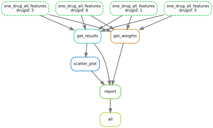
Imagine the case where you have 4 drugs, then results and weights are computed for each drug. This is parallelised on a distributed-computer. Once the computation is performed, a report is created.
The path of those files can be obtained using
from gdsctools import gdsctools_data
gdsctools_data("regression.rules", "../pipelines")
gdsctools_data("regression.yaml", "../pipelines")
Those two files must be copied in a local directory.
Then, edit the config file that looks like:
regression:
    method: lasso
    kfold: 10
    randomness: 50

input:
    ic50:
    genomic_features:
so as to set the input IC50 and genomic_features files. Once done, you can run the analysis. Just type:
snakemake -s regression.rules -j 4
Or a cluster, you may add the following information (for instance on a slurm system):
snakemake -s regression.rules -j 40 --cluster "sbatch --qos normal"
where -j 40 means uses 40 cores. Wait until it is finished. You should have an index.html file at the end.
Note
There is a standalone that fetches the pipeline and its config file, autofilled with user’s argument ready to run. The standalone is called gdsctools_regression. Please see Standalone application section