14. References
Contents
14.1. ANOVA related
14.1.1. The ANOVA analysis
Code related to the ANOVA analysis to find associations between drug IC50s and genomic features
-
class
ANOVA(ic50, genomic_features=None, drug_decode=None, verbose=True, set_media_factor=False)[source]¶ ANOVA analysis of the IC50 vs Feature matrices
This class is the core of the analysis. It can be used to compute
- One association between a drug and a feature
- The association**S** between a drug and a set of features
- All assocations between a set of drugs and a set of features.
For instance here below, we read an IC50 matrix and compute the association for a given drug with a specific feature.
Note that genomic features are not provided as input but a default file is provided with this package that contains 49 genomic features for 988 cell lines. If your IC50 contains unknown cell lines, you can provide your own file or use the
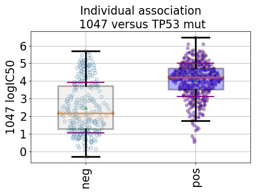
gdsctools.datasetsv17.from gdsctools import IC50, ANOVA, ic50_test ic = IC50(ic50_test) an = ANOVA(ic) # This is to select a specific tissue an.set_cancer_type('breast') df = an.anova_one_drug_one_feature(1047, 'TP53_mut', show=True)
(Source code, png, hires.png, pdf)

Details about the anova analysis: In the example above, we perform a regression/anova test based on OLS regression. This is done for one feature one drug across all cell lines (tissue) in the method
anova_one_drug(). The regression takes into account the following factors: tissue, MSI, MEDIA and features. If there is only one tissue, this factor is dropped. If the number of MSI values is less than a pre-defined parameter (seeANOVASettings), it is dropped. MEDIA, MSI columns are optional. The other methodsanova_one_drug()andanova_all()are wrappers aroundanova_one_drug_one_feature()to loop over all drugs, and loop over all drugs and all features, respectively.Please see the online documentation (ANOVA sections) for more help on gdsctools.readthedocs.io
Specific notes about the parameters. Default settings are used except for those releases:
V17
gdsc.volcano_FDR_interpolation = False
gdsc.settings.pvalue_correction_method = 'qvalue'
V18
gdsc.settings.FDR_threshold = 35
Constructor
Parameters: - IC50 (DataFrame) – a dataframe with the IC50. Rows should be the COSMIC identifiers and columns should be the Drug names (or identifiers)
- features – another dataframe with rows as in the IC50 matrix and columns as features. The first 3 columns must be named specifically to hold tissues, MSI (see format).
- drug_decode – a 3 column CSV file with drug’s name and targets
see
readersfor more information. - verbose – verbosity in “WARNING”, “ERROR”, “DEBUG”, “INFO”
Please see
readersmodule for details about the input formats.The
settingsattribute contains specific settings related to the ANOVA analysis or visualisation.-
add_pvalues_correction(df, colname='ANOVA_FEATURE_pval')[source]¶ Compute and add corrected pvalues in column ANOVA_FEATURE_FDR
Parameters: - df – a dataframe with a column named after colname (defaults to
ANOVA_FEATURE_pval). The output of
anova_all()contains such a dataframe. - colname (str) – name of the column that contains the pvalues to be corrected.
The default multiple testing correction (FDR correction) is stored in
settings.pvalue_correction_methodand can be changed to other methods (e.g., qvalue).The results in stored in a column named ANOVA_FEATURE_FDR inside the input dataframe df.
Values are in the range 0 to 1.
See also
- df – a dataframe with a column named after colname (defaults to
ANOVA_FEATURE_pval). The output of
-
anova_all(animate=True, drugs=None, multicore=None)[source]¶ Run all ANOVA tests for all drugs and all features.
Parameters: - drugs – you may select a subset of drugs
- animate – shows the progress bar
Returns: an
ANOVAResultsinstance with the dataframe stored in an attribute called dfCalls
anova_one_drug()for each drug and concatenate all results together. Note that once all data are gathered,add_pvalues_correction()is called to fill a new column with FDR corrections.An extra column named “ASSOC_ID” is also added with a unique identifer sorted by ascending FDR.
Note
A thorough comparison with version v17 gives the same FDR results (difference ~1e-6); Note however that the qvalue results differ by about 0.3% due to different smoothing in R and Python.
-
anova_one_drug(drug_id, animate=True, output='object')[source]¶ Computes ANOVA for a given drug across all features
Parameters: - drug_id (str) – a valid drug identifier.
- animate – shows the progress bar
Returns: a dataframe
Calls
anova_one_drug_one_feature()for each feature.
-
anova_one_drug_one_feature(drug_id, feature_name, show=False, production=False, directory='.', fontsize=18)[source]¶ Compute ABOVA one drug and one feature level
Parameters: - drug_id – a valid drug identifier
- feature_name – a valid feature name
- show (bool) – show boxplots with the different factor used
- directory (str) – where to save the figure.
- production (bool) – if False, returns a dataframe otherwise a dictionary. This is to speed up analysis when scanning the drug across all features.
Note
for developer this is the core of the analysis and should be kept as fast as possible. 95% of the time is spent here.
Note
for developer Data used in this function comes from _get_one_drug_one_feature_data method, which should also be kept as fast as possible.
-
anova_one_drug_one_feature_custom(drug_id, feature_name, formula, odof=None)[source]¶ Same as
anova_one_drug_one_feature()but allows any formulaReturns: full ANOVA table but also populate interal attribute anova_pvalues that is a dictionary with pvalues for feature, media, msi and tissue Formula must be set in the settings attribute as follows:
an = ANOVA(...)
an.settings['regression_formula'] = "Y ~  C(tissue) + feature"
Note
This function is convenient but 3-4 times slower than
anova_one_drug_one_feature(). So if your formula are one of:"Y ~ C(tissue) + C(media) + C(msi) + feature" "Y ~ C(tissue) + C(msi) + feature" "Y ~ C(msi) + feature" "Y ~ feature"
you should rather use
anova_one_drug_one_feature()instead (keeping regression_formula set to ‘auto’).By default, in categories, the first treatment (e.g tissue) is used as a reference and is not shown in the results. You may set the reference as follows:
"Y ~ C(tissue, Treatment(reference='breast'))"ANOVA pvalues returned are of type I
New in version 0.15.0.
-
reset_buffer()[source]¶ Reset the buffer used to store the results
When calling
anova_all(), the methodanova_one_drug()is called for each drug and the results saved in theindividual_anovaattribute. If called again, the results are simply returned from the buffer and not recomputed.If you change a settings that affects the analysis and therefore the results, then you should call this method.
14.1.2. The ANOVA results
ANOVAResults data structure to store the output of the ANOVA analysis
-
class
ANOVAResults(filename=None, settings=None)[source]¶ Class to handle results of the ANOVA analysis
The
ANOVAclass and in particular its methodanova_all()returns the results of the ANOVA analysis for each drug and genomic feature. The results are stored in a data structure defined in this class, which is just a dataframe stored indfattribute with the following header:Column name Description ASSOC_ID Alphanumeric identifier of the interaction FEATURE The CFE involved in the interaction, it can be a mutated cancer driver gene (CG) [suffix _mut], an abberrantly fused protein [suffix fusion], a copy number altered chromosomal region (RACS) [prefix gain for amplifications or loss for deletions]; DRUG_ID Numerical id of the drug involved in the interaction; DRUG_TARGET Putative target of the drug involved in the interaction; N_FEATURE_pos Number of cell lines harbouring the CFE indicated in column E and that have been screened with the drug indicated in columns F and G, therefore have been included in the test; N_FEATURE_neg Number of cell lines not harbouring the CFE indicated in column E and that have been screened with the drug indicated in columns F and G, therefore have been included in the test; FEATURE_pos_logIC50_MEAN Average log IC50 of the population of cell lines accounted in colum i; FEATURE_neg_logIC50_MEAN Average log IC50 of the population of cell lines accounted in colum j; FEATURE_delta_MEAN_IC50 Difference between the two average natural log IC50 values in the previous two columns (j - i). A negative value indicates an interaction for sensitivity, whereas a positive value indicates an interaction for resistance; FEATURE_pos_IC50_sd Log IC50 Standard deviation for the population of cell lines accounted in column i; FEATURE_neg_IC50_sd Log IC50 Standard deviation for the population of cell lines accounted in column j; FEATURE_IC50_effect_size Cohen’s d, quantifying the effect size of the interaction. A value >=0.5 indicates a moderate effect size. A value >=1 indicates a large effect size (i.e. difference in mean log IC50 values greater than their pooled standard deviations). A value >= 2 indicates a very large effect size (i.e. difference in mean log IC50 is at least two times their pooled standard deviation); FEATURE_pos_Glass_delta Glass delta, quantifying the effect size of the interaction as the ratio between the difference of the mean log IC50 values and the standard deviation of the log IC50 values of the population of cell lines accounted in column i; FEATURE_neg_Glass_delta Glass delta Same as above for the negative set. ANOVA_FEATURE_pval ANOVA test p-value quantyfing the interaction significance; ANOVA_TISSUE_pval ANOVA test p-value quantifying the significance of the interaction between drug response and the tissue of origin of the cell lines; for the cancer-specific interactions this value is NA; ANOVA_MEDIA_pval ANOVA test p-value quantifying the significance of the interaction between drug response and the screening medium of the cell lines; for the cancer-specific interactions this value is NA; ANOVA_MSI_pval ANOVA test p-value quantifying the significance of the interaction between drug response and the micro-satellite instability status of the cell lines; for the cancer type with no micro-satellite instable cell line samples this value is NA; ANOVA_FEATURE_FDR False discovery rate obtained by correcting the p-values in column u, on an individual analysis basis, for multiple hypothesis testing with the q-value correction method (Storey & TIbshirani, 2003) Note that those column names are renamed internally (and if the data is saved in a new file):
assoc_id ASSOC_ID Drug id DRUG_ID Owned_by OWNED_BY FEATUREpos_IC50_sd FEATURE_pos_IC50_sd FEATUREneg_IC50_sd FEATURE_neg_IC50_sd FEATUREpos_Glass_delta FEATURE_pos_Glass_delta FEATUREneg_Glass_delta FEATURE_neg_Glass_delta FEATUREpos_logIC50_MEAN FEATURE_pos_logIC50_MEAN FEATUREneg_logIC50_MEAN FEATURE_neg_logIC50_MEAN Drug Target DRUG_TARGET FEATURE_deltaMEAN_IC50 FEATURE_delta_MEAN_IC50 FEATURE_ANOVA_pval ANOVA_FEATURE_pval ANOVA FEATURE FDR % ANOVA_FEATURE_FDR MSI_ANOVA_pval ANOVA_MSI_pval Tissue_ANOVA_pval ANOVA_TISSUE_pval MEDIA_ANOVA_pval ANOVA_MEDIA_pval TISSUE_ANOVA_pval ANOVA_TISSUE_pval Drug name DRUG_NAME Constructor
Parameters: filename (str) – Another ANOVAResults instance or a compatible CSV file with the correct header. The filename may also be set to None (default) and populated later. -
df¶ dataframe with all results
-
drugIds¶ Returns the list of drug identifiers
-
get_html_table(collapse_table=False, clip_threshold=2, index=False, header=True, escape=False, add_href=True)[source]¶ Return an HTML table for the reports
Parameters: add_href – add href to the FEATURE, DRUG ID and ASSOC ID
-
mapping= None¶ dictionary with the relevant column names and their expected types
-
14.1.3. The ANOVA report
Code related to the ANOVA analysis to find associations between drug IC50s and genomic features
-
class
ANOVAReport(gdsc, results=None, sep='t', drug_decode=None, verbose=True)[source]¶ Class used to interpret the results and create final HTML report
Results is a data structure returned by
ANOVA.anova_all().from gdsctools import * # Perform the analysis itself to get a set of results (dataframe) an = ANOVA(ic50_test) results = an.anova_all() # now, we can create the report. r = ANOVAReport(gdsc=an, results=results) # we can tune some settings r.settings.pvalue_threshold = 0.001 r.settings.FDR_threshold = 28 r.settings.directory = 'testing' r.create_html_pages()
Significant association
An association is significant if
- The field ANOVA_FEATURE_FDR must be < FDR_threshold
- The field ANOVA_FEATURE_pval must be < pvalue_threshold
It is then labelled sensible if FEATURE_delta_MEAN_IC50 is below 0, otherwise it is resistant.
Constructor
Parameters: - gdsc – the instance with which you created the results to report
- results – the results returned by
ANOVA.anova_all(). If not provided, the ANOVA is run on the fly.
-
create_html_associations()[source]¶ Create an HTML page for each significant association
The name of the output HTML file is <association id>.html where association id is stored in
df.
-
create_html_manova(onweb=True)[source]¶ Create summary table with all significant hits
Parameters: onweb – open browser with the created HTML page.
-
drug_summary(top=50, fontsize=15, filename=None)[source]¶ Return dataframe with significant drugs and plot figure
Parameters: - fontsize –
- top – max number of significant associations to show
- filename – if provided, save the file in the directory
-
feature_summary(filename=None, top=50, fontsize=15)[source]¶ Return dataframe with significant features and plot figure
Parameters: - fontsize –
- top – max number of significant associations to show
- filename – if provided, save the file in the directory
-
get_significant_hits(show=True)[source]¶ Return a summary of significant hits
Parameters: show – show a plot with the distribution of significant hits Todo
to finalise
-
n_celllines¶ return number of cell lines
-
n_drugs¶ return number of drugs
-
n_tests
14.2. Statistical Tools
Code related to the ANOVA analysis to find associations between drug IC50s and genomic features
-
class
MultipleTesting(method=None)[source]¶ This class eases the computation of multiple testing corrections
The method implemented so far are based on statsmodels or a local implementation of qvalue method.
method name Description bonferroni one-step correction sidak one-step correction holm-sidak step down method using Sidak adjustments holm step down method using Bonferroni adjustments simes-hochberg step up method (independent) hommel close method based on Simes tests (non negative) fdr_bh FDR Benjamini-Hochberg (non-negative) fdr_by FDR Benjamini-Yekutieli (negative) fdr_tsbky FDR 2-stage Benjamini-Krieger-Yekutieli non negative frd_tsbh FDR 2-stage Benjamini-Hochberg’ non-negative fdr same as fdr_bh qvalue see QValueclassSee also
Constructor
Parameters: method – default to fdr that is the FDR Benjamini-Hochberg correction. -
get_corrected_pvalues(pvalues, method=None)[source]¶ Return corrected pvalues
Parameters: - pvalues (list) – list or array of pvalues to correct.
- method – use the one defined in the constructor by default but can be overwritten here
-
method¶ get/set method
-
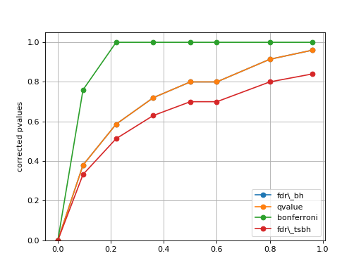
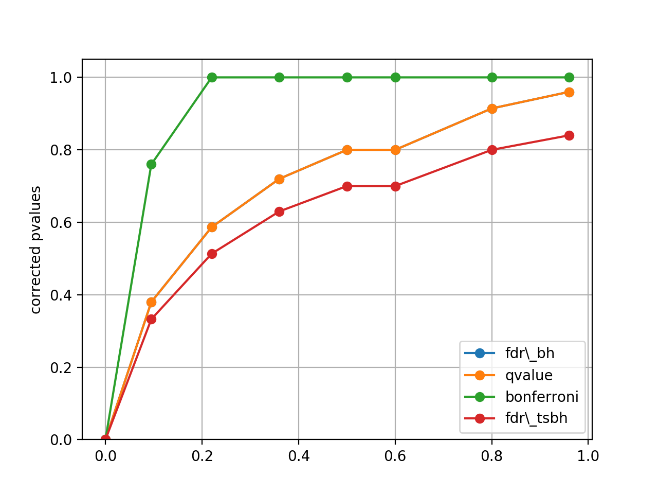
plot_comparison(pvalues, methods=None)[source]¶ Simple plot to compare the pvalues correction methods
from gdsctools.stats import MultipleTesting
mt = MultipleTesting()
pvalues = [1e-10, 9.5e-2, 2.2e-1, 3.6e-1, 5e-1, 6e-1,8e-1,9.6e-1]
mt.plot_comparison(pvalues,
    methods=['fdr_bh', 'qvalue', 'bonferroni', 'fdr_tsbh'])
(Source code, png, hires.png, pdf)

Note
in that example, the qvalue and FDR are identical, but this is not true in general.
-
valid_methods= None¶ set of valid methods
-
-
cohens(x, y)[source]¶ Effect size metric through Cohen’s d metric
Parameters: - x – first vector
- y – second vector
Returns: absolute effect size value
The Cohen’s effect size d is defined as the difference between two means divided by a standard deviation of the data.

For two independent samples, the pooled standard deviation is used instead, which is defined as:
A Cohen’s d is frequently used in estimating sample sizes for statistical testing: a lower d value indicates the necessity of larger sample sizes, and vice versa.
Note
we return the absolute value
References: https://en.wikipedia.org/wiki/Effect_size
Implementation of qvalue estimate
Author: Thomas Cokelaer
-
class
QValue(pv, lambdas=None, pi0=None, df=3, method='smoother', smooth_log_pi0=False, verbose=True)[source]¶ Compute Q-value for a given set of P-values
Constructor
The q-value of a test measures the proportion of false positives incurred (called the false discovery rate or FDR) when that particular test is called significant.
Parameters: - pv – A vector of p-values (only necessary input)
- lambdas – The value of the tuning parameter to estimate pi_0. Must be in [0,1). Can be a single value or a range of values. If none, the default is a range from 0 to 0.9 with a step size of 0.05 (inluding 0 and 0.9)
- method – Either “smoother” or “bootstrap”; the method for automatically choosing tuning parameter in the estimation of pi_0, the proportion of true null hypotheses. Only smoother implemented for now.
- df – Number of degrees-of-freedom to use when estimating pi_0 with a smoother (default to 3 i.e., cubic interpolation.)
- pi0 (float) – if None, it’s estimated as suggested in Storey and Tibshirani, 2003. May be provided, which is convenient for testing.
- smooth_log_pi0 – If True and ‘pi0_method’ = “smoother”, pi_0 will be estimated by applying a smoother to a scatterplot of log pi_0 rather than just pi_0
Note
Estimation of pi0 differs slightly from the one given in R (about 0.3%) due to smoothing.spline function differences between R and SciPy.
If no options are selected, then the method used to estimate pi_0 is the smoother method described in Storey and Tibshirani (2003). The bootstrap method is described in Storey, Taylor & Siegmund (2004) but not implemented yet.
See also
14.3. Readers
14.3.1. IC50, Genomic Features, Drug Decode
IO functionalities
Provides readers to read the following formats
- Matrix of IC50 data set
IC50 - Matrix of Genomic features with
GenomicFeatures - Drug Decoder table with
DrugDecode
-
class
IC50(filename, v18=False)[source]¶ Reader of IC50 data set
This input matrix must be a comman-separated value (CSV) or tab-separated value file (TSV).
The matrix must have a header and at least 2 columns. If the number of rows is not sufficient, analysis may not be possible.
The header must have a column called “COSMIC_ID” or “COSMIC ID”. This column will be used as indices (row names). All other columns will be considered as input data.
The column “COSMIC_ID” contains the cosmic identifiers (cell line). The other columns should be filled with the IC50s corresponding to a pair of COSMIC identifiers and Drug. Nothing prevents you to fill the file with data that have other meaning (e.g. AUC).
If at least one column starts with
Drug_, all other columns will be ignored. This was implemented for back compatibility.The order of the columns is not important.
Here is a simple example of a valid TSV file:
COSMIC_ID   Drug_1_IC50 Drug_20_IC50
111111      0.5         0.8
222222      1           2
A test file is provided in the gdsctools package:
from gdsctools import ic50_test
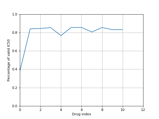
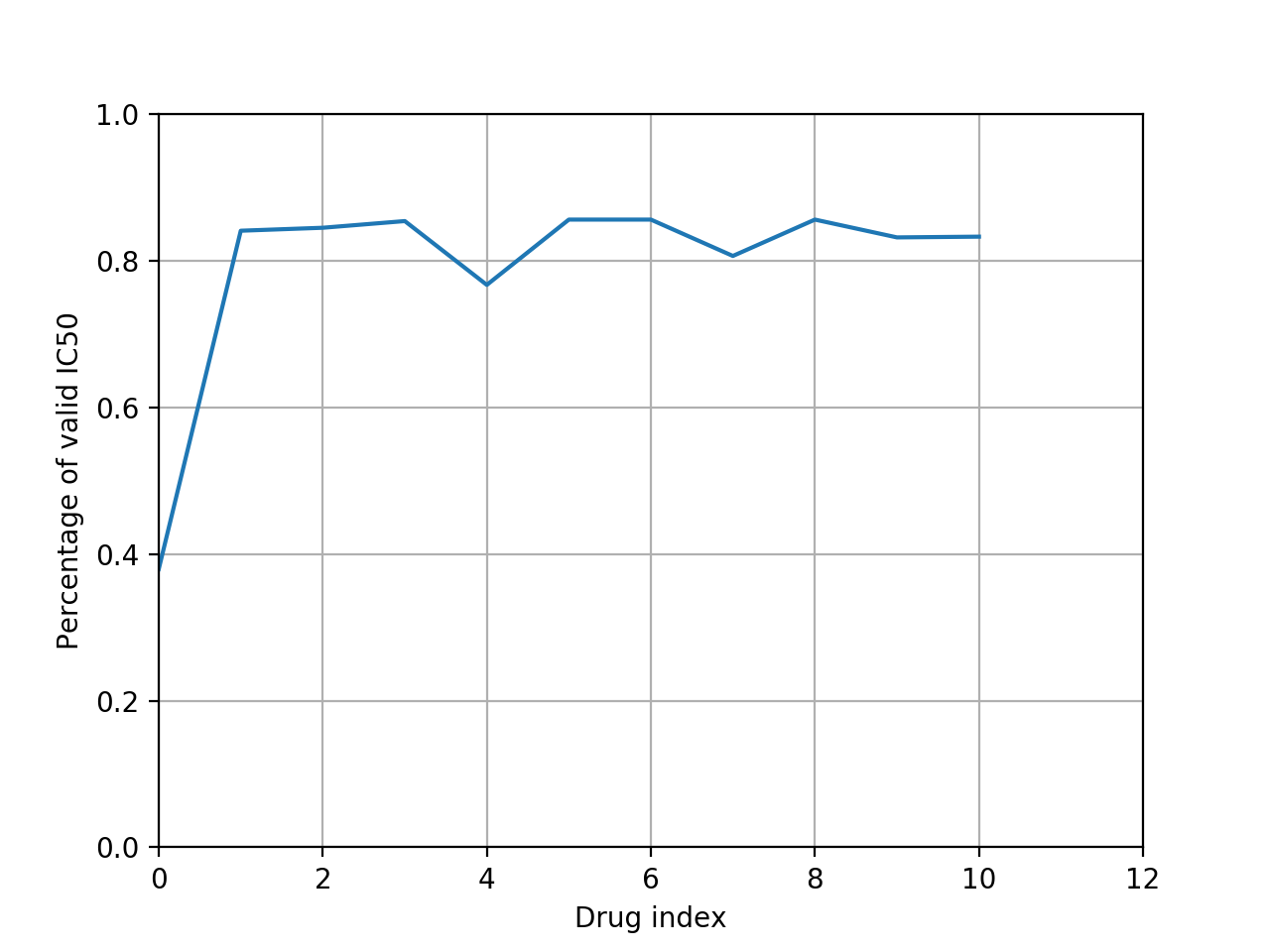
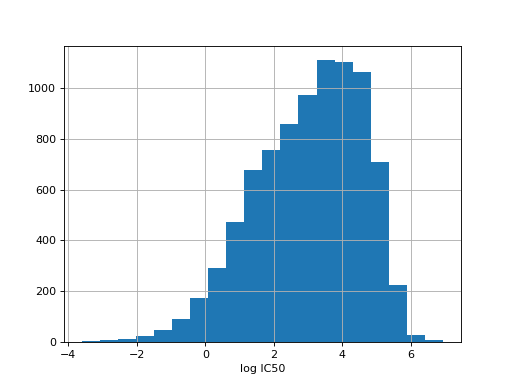
You can read it using this class and plot information as follows:
from gdsctools import IC50, ic50_test
r = IC50(ic50_test)
r.plot_ic50_count()
(Source code, png, hires.png, pdf)
You can get basic information using the print function:
>>> from gdsctools import IC50, ic50_test
>>> r = IC50(ic50_test)
>>> print(r)
Number of drugs: 11
Number of cell lines: 988
Percentage of NA 0.206569746043
You can get the drug identifiers as follows:
r.drugIds
and set the drugs, which means other will be removed:
r.drugsIds = [1, 1000]
Changed in version 0.9.10: The column COSMIC ID should now be COSMIC_ID. Previous name is deprecated but still accepted.
Constructor
Parameters: filename – input filename of IC50s. May also be an instance of IC50or a valid dataframe. The data is stored as a dataframe in the attribute calleddf. Input file may be gzipped-
cosmic_name= 'COSMIC_ID'
-
drugIds¶ list the drug identifier name or select sub set
-

-
class
GenomicFeatures(filename=None, empty_tissue_name='UNDEFINED')[source]¶ Read Matrix with Genomic Features
These are the compulsary column names required (note the spaces):
- ‘COSMIC_ID’
- ‘TISSUE_FACTOR’
- ‘MSI_FACTOR’
If one of the following column is found, it is removed (deprecated):
- 'SAMPLE_NAME'
- 'Sample Name'
- 'CELL_LINE'
and features can be also encoded with the following convention:
- columns ending in “_mut” to encode a gene mutation (e.g., BRAF_mut)
- columns starting with “gain_cna”
- columns starting with “loss_cna”
Those columns will be removed:
- starting with Drug_, which are supposibly from the IC50 matrix
>>> from gdsctools import GenomicFeatures
>>> gf = GenomicFeatures()
>>> print(gf)
Genomic features distribution
Number of unique tissues 27
Number of unique features 677 with
- Mutation: 270
- CNA (gain): 116
- CNA (loss): 291
Changed in version 0.9.10: The header’s columns’ names have changed to be more consistant. Previous names are deprecated but still accepted.
Changed in version 0.9.15: If a tissue is empty, it is replaced by UNDEFINED. We also strip the spaces to make sure there is “THIS” and “THIS ” are the same.
Constructor
If no file is provided, using the default file provided in the package that is made of 1001 cell lines times 680 features.
Parameters: empty_tissue_name (str) – if a tissue name is let empty, replace it with this string. -
colnames= {'cosmic': 'COSMIC_ID', 'media': 'MEDIA_FACTOR', 'msi': 'MSI_FACTOR', 'tissue': 'TISSUE_FACTOR'}
-
compress_identical_features()[source]¶ Merge duplicated columns/features
Columns duplicated are merged as follows. Fhe first column is kept, others are dropped but to keep track of those dropped, the column name is renamed by concatenating the columns’s names. The separator is a double underscore.
gf = GenomicFeatures()
gf.compress_identical_features()
# You can now access to the column as follows (arbitrary example)
gf.df['ARHGAP26_mut__G3BP2_mut']
-
drop_tissue_in(tissues)[source]¶ Drop tissues from the list
Parameters: tissues (list) – a list of tissues to drop. If you have only one tissue, can be provided as a string. Since rows are removed some features (columns) may now be empty (all zeros). If so, those columns are dropped (except for the special columns (e.g, MSI).
-
features¶ return list of features
-
fill_media_factor()[source]¶ Given the COSMIC identifiers, fills the MEDIA_FACTOR column
If already populated, replaced by new content.
-
keep_tissue_in(tissues)[source]¶ Drop tissues not in the list
Parameters: tissues (list) – a list of tissues to keep. If you have only one tissue, can be provided as a string. Since rows are removed some features (columns) may now be empty (all zeros). If so, those columns are dropped (except for the special columns (e.g, MSI).
-
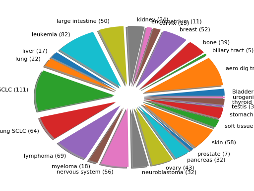
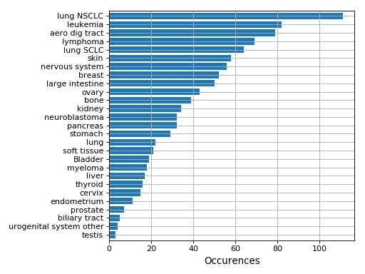
plot(shadow=True, explode=True, fontsize=12)[source]¶ Histogram of the tissues found
from gdsctools import GenomicFeatures
gf = GenomicFeatures() # use the default file
gf.plot()
-
shift
-
tissues¶ return list of tissues
-
unique_tissues¶ return set of tissues
-
class
Reader(data=None)[source]¶ Convenience base class to read CSV or TSV files (using extension)
Constructor
This class takes only one input parameter, however, it may be a filename, or a dataframe or an instance of
Readeritself. This means than children classes such asIC50can also be used as input as long as a dataframe nameddfcan be found.Parameters: data – a filename in CSV or TSV format with format specified by child class (see e.g. IC50), or a valid dataframe, or an instance ofReader.The input can be a filename either in CSV (comma separated values) or TSV (tabular separated values). The extension will be used to interpret the content, so please be consistent in the naming of the file extensions.
>>> from gdsctools import Reader, ic50_test
>>> r = Reader(ic50_test.filename) # this is a CSV file
>>> len(r.df)   # number of rows
988
>>> len(r)      # number of elements
11856
Note that
Readeris a base class and more sophisticated readers are available. for example, theIC50would be better to read this IC50 data set.The data has been stored in a data frame in the
dfattribute.The dataframe of the object itself can be used as an input to create an new instance:
>>> from gdsctools import Reader, ic50_test
>>> r = Reader(ic50_test.filename, sep="\t")
>>> r2 = Reader(r) # here r.df is simply copied into r2
>>> r == r2
True
It is sometimes convenient to create an empty Reader that will be populated later on:
>>> r = Reader()
>>> len(r)
0
More advanced readers (e.g.
IC50) can also be used as input as long as they have adfattribute:>>> from gdsctools import Reader, ic50_test >>> ic = IC50(ic50_test) >>> r = Reader(ic)
-
check()[source]¶ Checking the format of the matrix
Currently, only checks that there is no duplicated column names
-
header= None¶ if populated, can be used to check validity of a header
-
-
class
DrugDecode(filename=None)[source]¶ Reads a “drug decode” file
The format must be comma-separated file. There are 3 compulsary columns called DRUG_ID, DRUG_NAME and DRUG_TARGET. Here is an example:
DRUG_ID     ,DRUG_NAME   ,DRUG_TARGET
999         ,Erlotinib   ,EGFR
1039        ,SL 0101-1   ,"RSK, AURKB, PIM3"
TSV file may also work out of the box. If a column name called ‘PUTATIVE_TARGET’ is found, it is renamed ‘DRUG_TARGET’ to be compatible with earlier formats.
In addition, 3 extra columns may be provided:
- PUBCHEM_ID
- WEBRELEASE
- OWNED_BY
The OWNED_BY and WEBRELEASE may be required to create packages for each company. If those columns are not provided, the internal dataframe is filled with None.
Note that older version of identifiers such as:
Drug_950_IC50are transformed as proper ID that is (in this case), just the number:
950Then, the data is accessible as a dataframe, the index being the DRUG_ID column:
data = DrugDecode('DRUG_DECODE.csv')
data.df.iloc[999]
Note
the DRUG_ID column must be made of integer
Constructor
-
companies
-
drugIds¶ return list of drug identifiers
-
drug_annotations(df)[source]¶ Populate the drug_name and drug_target field if possible
Parameters: df – input dataframe as given by e.g., anova_one_drug()Return df: same as input but with the FDR column populated
-
drug_names
-
drug_targets
-
14.3.2. OmniBEM related
OmniBEM functions
-
class
OmniBEMBuilder(genomic_alteration)[source]¶ Utility to create
GenomicFeaturesinstance from BEM dataStarting from an example provided in GDSCTools (test_omnibem_genomic_alteration.csv.gz), here is the code to get a data structure compatible with the
GenomicFeature, which can then be used as input to theANOVAclass.See the constructor for the header format.
from gdsctools import gdsctools_data, OmniBEMBuilder, GenomicFeatures

input_data = gdsctools_data("test_omnibem_genomic_alterations.csv.gz")
bem = OmniBEMBuilder(input_data)

# You may filter the data for instance to keep only a set of genes.
# Here, we keep everything
gene_list = bem.df.GENE.unique()
bem.filter_by_gene_list(gene_list)

# Finally, create a MoBEM dataframe
mobem = bem.get_mobem()

# You may filter with other functions(e.g., to keep only Methylation
# features
bem.filter_by_type_list(["Methylation"])
mobem = bem.get_mobem()

# Then, let us create a dataframe that is compatible with
# GenomicFeature. We just need to make sure the columns are correct
mobem[[x for x in mobem.columns if x!="SAMPLE"]]
gf = GenomicFeatures(mobem[[x for x in mobem.columns if x!="SAMPLE"]])

# Now, we can perform an ANOVA analysis:
from gdsctools import ANOVA, ic50_test
an = ANOVA(ic50_test, gf)
results = an.anova_all()
results.volcano()
(Source code, png, hires.png, pdf)
Note
The underlying data is stored in the attribute
df.Constructor
Parameters: genomic_alteration (str) – a filename in CSV format (gzipped or not). The format is explained here below. The input must be a 5-columns CSV file with the following columns:
COSMIC_ID: an integer
TISSUE_TYPE: e.g. Methylation,
SAMPLE: this should correspond to the COSMID_ID
TYPE: Methylation,
GENE: gene name
IDENTIFIER: required for now but may be removed (rows can be
    used as identifier indeed
Warning
If GENE is set to NA, we drop it. In the resources shown in the example here above, this corresponds to 380 rows (out of 60703). Similarly, if TISSUE is NA, we also drop these rows that is about 3000 rows.
-
filter_by_cosmic_list(cosmic_list)[source]¶ Filter the data by cosmic identifers
Parameters: cosmic (list) – the cosmic identifiers to be kept. The data is updated in place.
-
filter_by_gene_list(genes, minimum_gene=3)[source]¶ Keeps only required genes
Parameters: - genes – a list of genes or a filename (a CSV file with a column named GENE).
- minimum_gene – genes with not enough entries are removed (defaults to 3)
-
filter_by_sample_list(sample_list)[source]¶ Filter the data by sample name
Parameters: tissue (list) – the samples to be kept. The data is updated in place.
-
filter_by_tissue_list(tissue_list)[source]¶ Filter the data by tissue
Parameters: tissue (list) – the tissues to be kept. The data is update in place.
-
filter_by_type_list(type_list)[source]¶ Filter the data by type
Parameters: tissue (list) – the types to be kept. The data is update in place. Here are some examples of types: Point.mutation, Amplification, Deletion, Methylation.
-
get_mobem()[source]¶ Return a dataframe compatible with ANOVA analysis
The returned object can be read by
GenomicFeatures.
-
get_significant_genes(N=20)[source]¶ Return most present genes
Parameters: N (int) – the maximum number of genes to return Returns: list of genes with the number of occurences The genes returned by be used to filter the data:
genes = bem.get_significant_genes(N=20)
bem.filter_by_gene_list(genes.index)
-
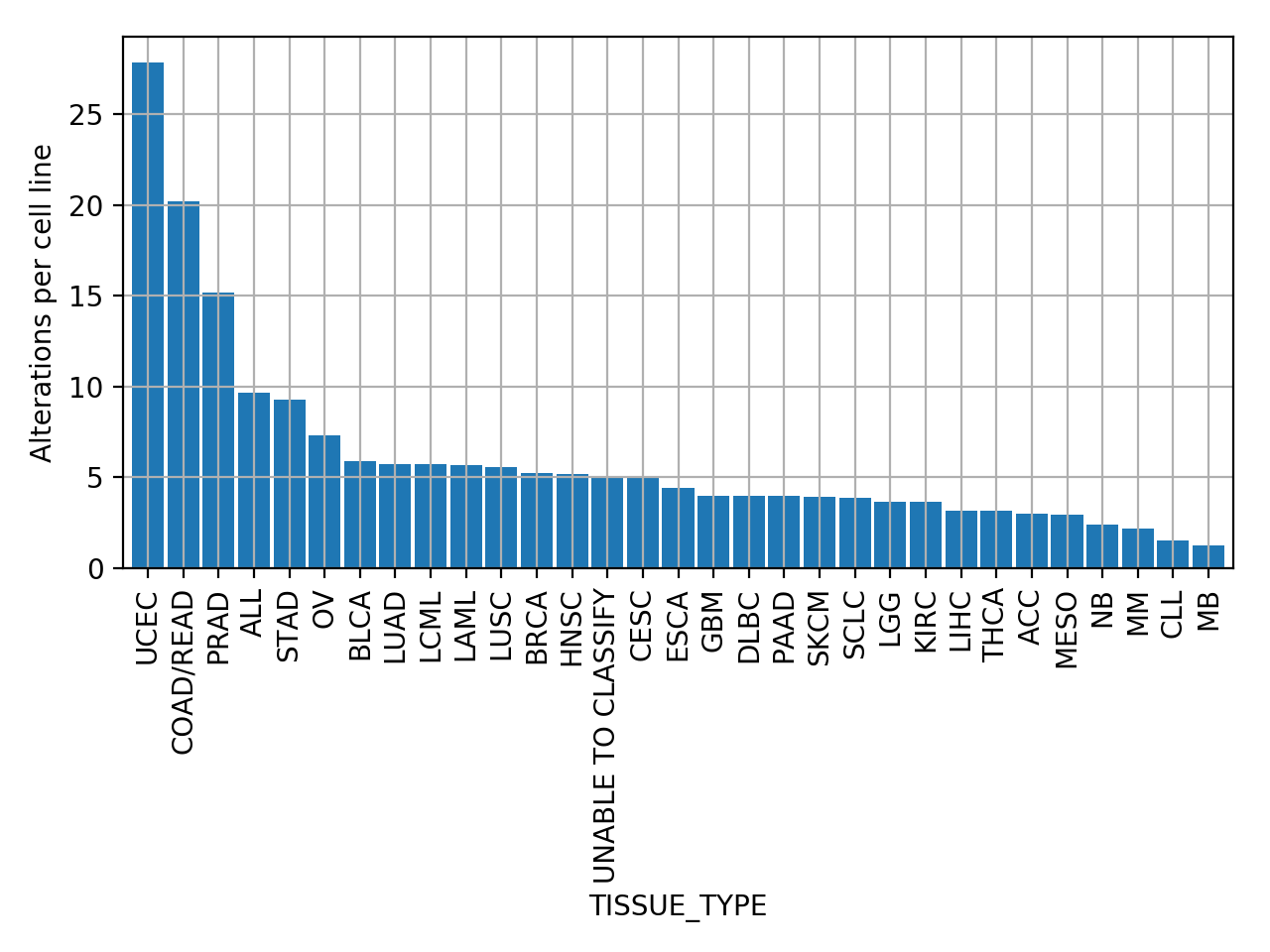
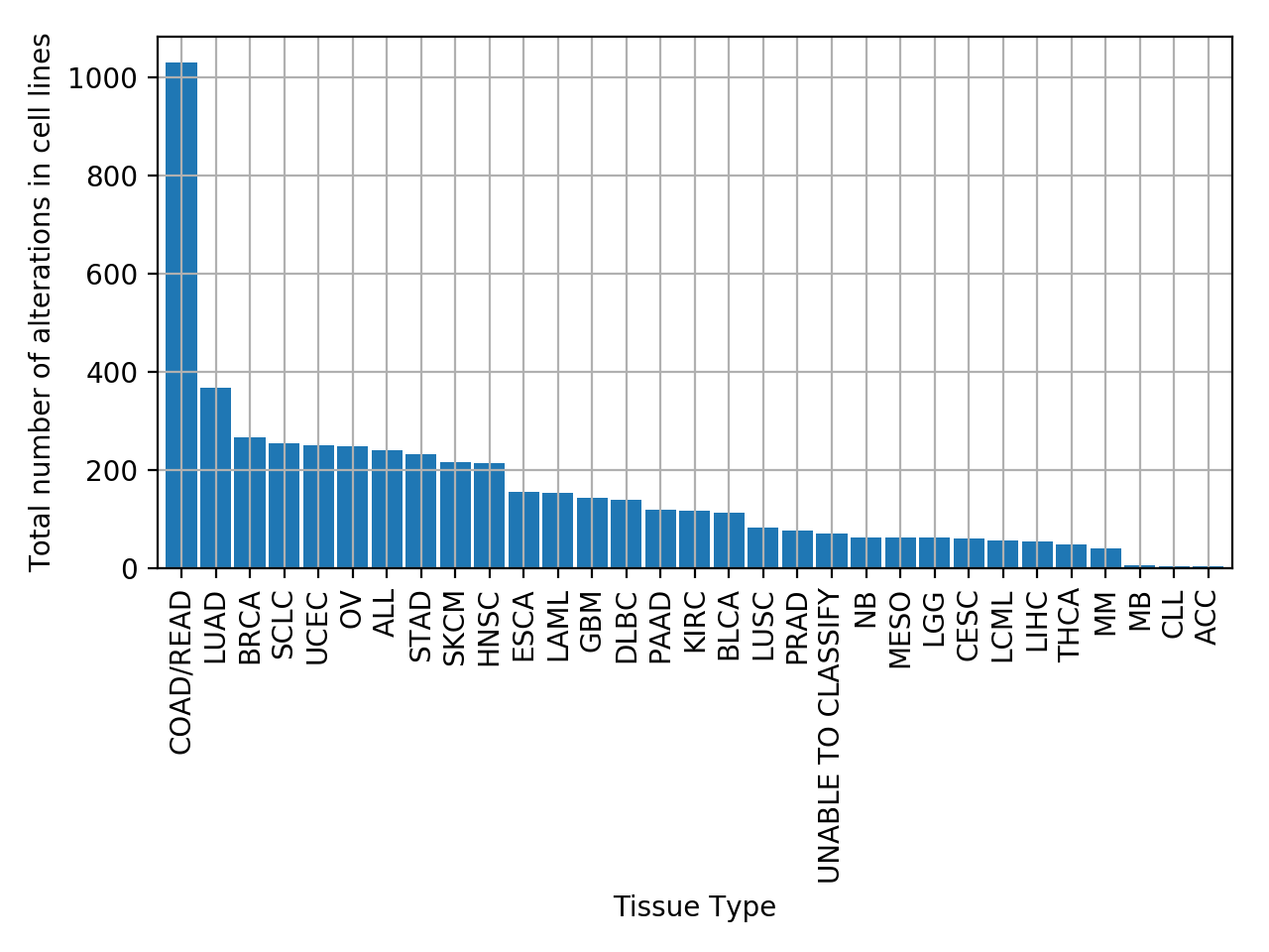
plot_alterations_per_cellline(fontsize=10, width=0.9)[source]¶ Plot number of alterations
from gdsctools import *
data = gdsctools_data("test_omnibem_genomic_alterations.csv.gz")
bem = OmniBEMBuilder(data)
bem.filter_by_gene_list(gdsctools_data("test_omnibem_genes.txt"))
bem.plot_alterations_per_cellline()
(Source code, png, hires.png, pdf)

-
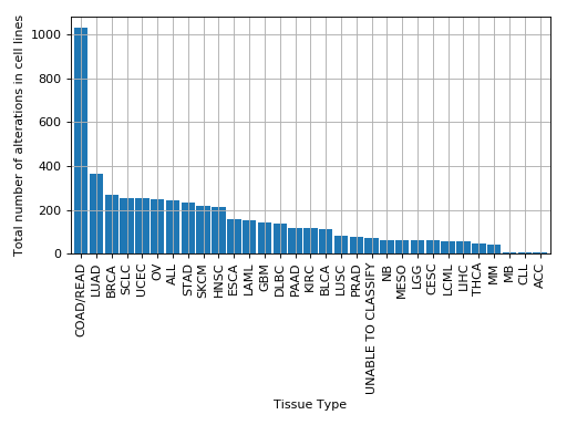
plot_number_alteration_by_tissue(fontsize=10, width=0.9)[source]¶ Plot number of alterations
from gdsctools import *
data = gdsctools_data("test_omnibem_genomic_alterations.csv.gz")
bem = OmniBEMBuilder(data)
bem.filter_by_gene_list(gdsctools_data("test_omnibem_genes.txt"))
bem.plot_number_alteration_by_tissue()
(Source code, png, hires.png, pdf)
-
This module provides an interface to download and filter GDSC1000 data, as published by Iorio et al (2016).
Author: Elisabeth D. Chen Date: 2016-06-17
-
class
GDSC1000(annotate=False, data_folder_name='./data/gdsc_1000_data/')[source]¶ Help data retrieval from GDSC website (version v17)
from gdsctools import GDSC1000
data = GDSC1000()
data.download_data()
Next time, starting GDSCTools in the same directory, just type:
data = GDSCTools()
data.load_data()
CNA (e.g.,
cna_df), Methylation and gene variants are downloaded. IC50 as well and a set of annotations. There are combined ingenomic_df.The
genomic_dfcontains thecna_df,methylation_dfandvariant_dfdata. The three latter contains in common the CELL_LINE, ALTERATION_TYPE, IDENTIFIER and TISSUE_FACTOR.ALTERATION_TYPE can be GENETIC_VARIATION, METHYLATION, DELETION / AMPLIFICATION variant_df also has the COSMIC_ID. The
annotation_dfgives mapping between identifiers and gene names.download_data()Download and load data in memory load_data([annotation])If CSV files are already downloaded, just load them make_matrix([min_recurrence])Return a dataframe compatible with ANOVA analysis With this class, you may (1) download the data, (2) annotate or filter the data and (3) create a genomic matrix.
To load the data, either download it from the website using
download_data()(downloads data from cancerrxgene.org loading methylation, cna, variant and cell lines datasets). It extract relevant columns, re-names column names and saves as csv files in thedata_folder_namedirectory.If you have already downloaded the data, you may just load it using
load_data(). This function also annotates the data with gene information.Then, you filter the data with one of the filter methods:
filter_by_cell_line([ "AsPC-1", "U-2-OS", "MDA-MB-231"... ] )
filter_by_cosmic_id([ 948121, 2839818, ...] )
filter_by_gene(["ATM", "TP53", ...])
filter_by_recurrence(min_recurrence = 3 )
filter_by_tissue_type([ "BRCA", "COAD/READ", ... ] )
filter_by_alteration_type(["METHYLATION", "AMPLIFICATION",
                                "DELETION", "GENE_VARIANT" ] )
Finally, you can create the genomic matrix using
make_matrix().You can also look at the unique regions for agiven data set. For instance, methylation dataframe has about 2,000 regions but only 338 are unique:
len(data.methylation_df.groupby('IDENTIFIER').groups)
constructor
Parameters: -
get_genomic_info()[source]¶ Return information about the genomic dataframe
The returned dataframes contains two columns: the number of unique cosmic identifiers and features for each type of alterations.
-
14.4. Visualisation
14.4.1. Volcano plot
Volcano plot utilities
The VolcanoANOVA is used in the creation of the report but
may be used by a usr in a Python shell.
-
class
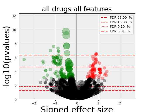
VolcanoANOVA(data, sep='t', settings=None)[source]¶ Utilities related to volcano plots
This class is used in
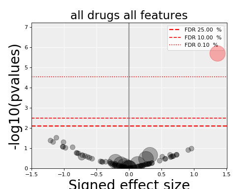
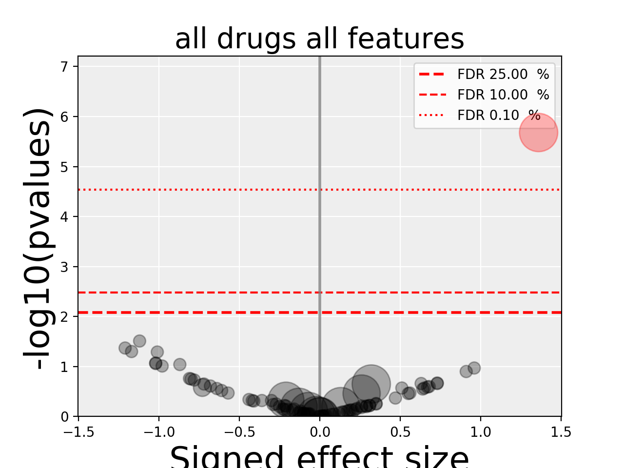
gdsctools.anovabut can also be used independently as in the example below.from gdsctools import ANOVA, ic50_test, VolcanoANOVA an = ANOVA(ic50_test) # retrict analysis to a tissue to speed up computation an.set_cancer_type('lung_NSCLC') # Perform the entire analysis results = an.anova_all() # Plot volcano plot of pvalues versus signed effect size v = VolcanoANOVA(results) v.volcano_plot_all()
(Source code, png, hires.png, pdf)

Note
Within an IPython shell, you should be able to click on a circle and the title will be updated with the name of the drug/feature and FDR value.
Legend and color conventions: The green circles indicate significant hits that are resistant while reds show sensitive hits. Circles are colored if there are below the FDR_threshold AND below the pvalue_threshold AND if the signed effect size is above the effect_threshold. Constructor
Parameters: - data – an
ANOVAResultsinstance or a dataframe with the proper columns names (see below) - settings – an instance of
ANOVASettings
Expected column names to be found if a filename is provided:
ANOVA_FEATURE_pval
ANOVA_FEATURE_FDR
FEATURE_delta_MEAN_IC50
FEATURE_IC50_effect_size
N_FEATURE_pos
N_FEATURE_pos
FEATURE
DRUG_ID
If the plotting is too slow, you can use the
selector()to prune the results (most of the data are noise and overlap on the middle bottom area of the plot with little information.-
selector(df, Nbest=1000, Nrandom=1000, inplace=False)[source]¶ Select only the first N best rows and N random ones
Sometimes, there are tens of thousands of associations and future analysis will include more features and drugs. Plotting volcano plots should therefore be fast and scalable. Here, we provide a naive way of speeding up the plotting by selecting only a subset of the data made of Nbest+Nrandom associations.
Parameters: Returns: pruned dataframe
-
volcano_plot_all()[source]¶ Create an overall volcano plot for all associations
This method saves the picture in a PNG file named volcano_all.png.
-
volcano_plot_all_drugs()[source]¶ Create a volcano plot for each drug and save in PNG files
Each filename is set to volcano_<drug identifier>.png
-
volcano_plot_all_features()[source]¶ Create a volcano plot for each feature and save in PNG files
Each filename is set to volcano_<feature name>.png
- data – an
14.4.2. Boxplot and beeswarm
-
boxswarm(data, names=None, vert=True, widths=0.5, **kwargs)[source]¶ Plot boxplot with all points as circles.
This function is a wrapper of
BoxSwarmParameters: - data – a dataframe. Each column is a data set from which a boxplot is created.
- names –
- vert – orientation of the boxplots
- widths – widths of the boxes
- kargs – any argument accepted by
BoxSwarm
See
BoxSwarmdocumentation for details
-
class
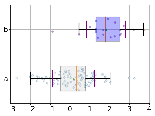
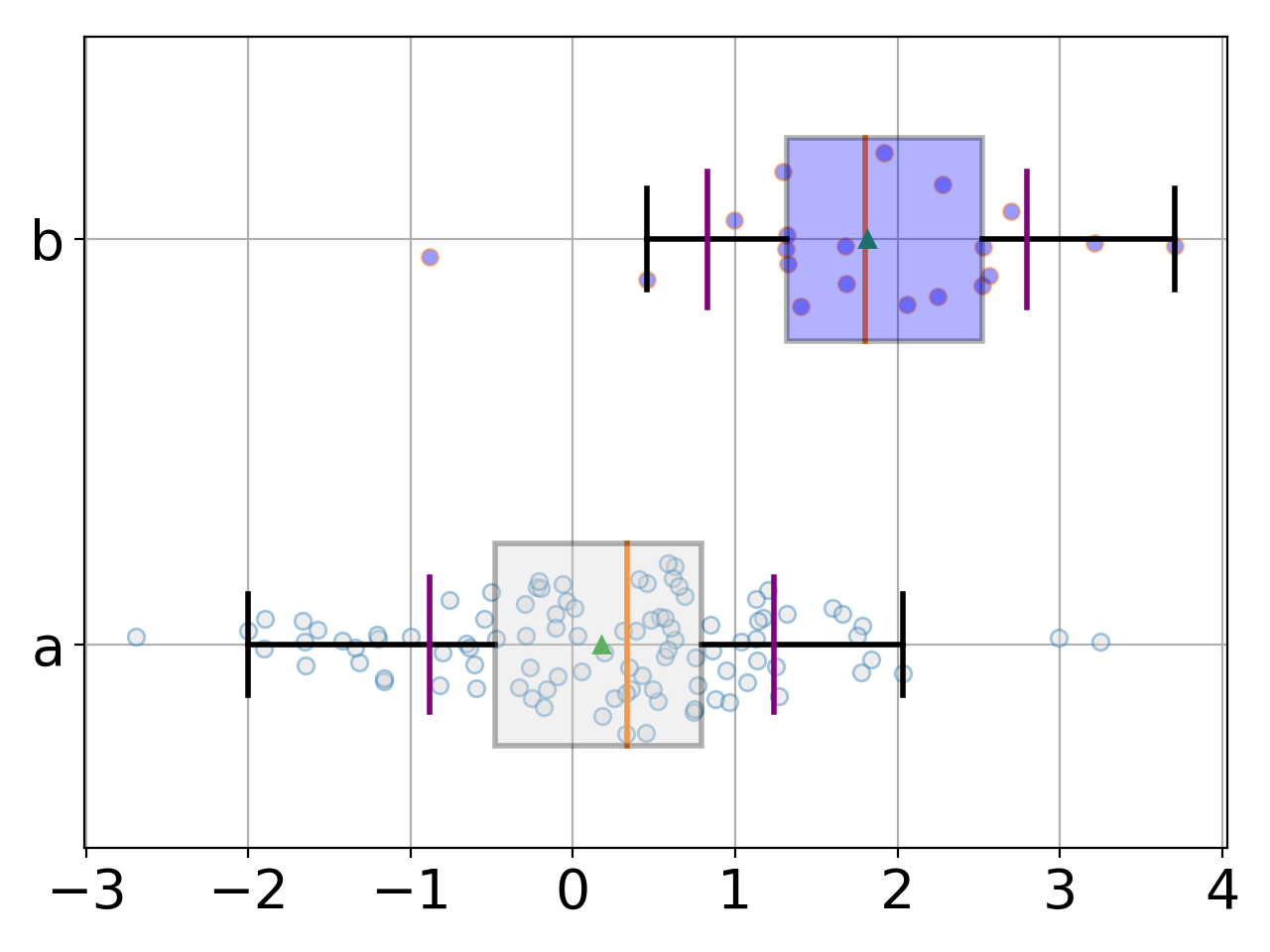
BoxSwarm(data, names=None, fontsize=20, hold=False, title='', lw=2, colors=['lightgrey', 'blue'])[source]¶ Simple beeswarm plot (boxplot + dots for each data point)
from pylab import randn
from gdsctools.boxswarm import BoxSwarm
b = BoxSwarm({'a':randn(100), 'b':randn(20)+2})
b.plot(vert=False)
(Source code, png, hires.png, pdf)

Note
could use pybeeswarm, which is a proper implementation of beeswarm.
Constructor
Param: a list of list (not same size) or a dictionary of lists
Parameters: - data –
- names –
- fontsize –
- hold –
- title –
- lw – width of lines
- colors – loop over the list of colors provided to fill boxplots
- **kargs –
-
beeswarm(data, position, ratio=2.0)[source]¶ Naive plotting of the data points
We assume gaussian distribution so we expect fewers dots far from the mean/median. We’d like those dots to be close to the axes. conversely, we expect lots of dots centered around the mean, in which case, we’d like them to be spread in the box. We uniformly distribute position using
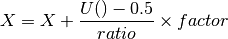
but the factor is based on an arctan function:
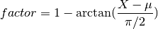
The farther the data is from the mean
 ,
the closest it is to the axes that goes through the box.
,
the closest it is to the axes that goes through the box.
Code related to the ANOVA analysis to find associations between drug IC50s and genomic features
-
class
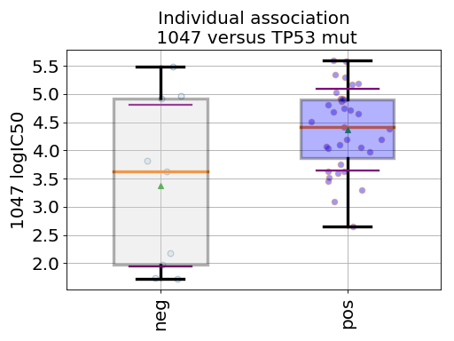
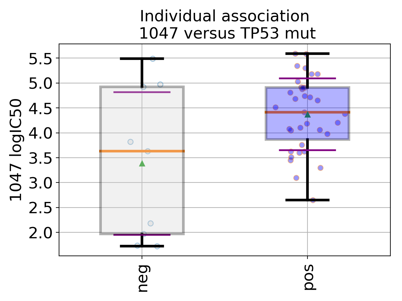
BoxPlots(odof, fontsize=20, savefig=False, directory='.')[source]¶ Box plot for a given association of drug versus genomic feature
from gdsctools import ANOVA, ic50_test
from gdsctools.boxplots import BoxPlots

gdsc = ANOVA(ic50_test)

# Perform the entire analysis
odof = gdsc._get_one_drug_one_feature_data(1047, 'TP53_mut')

# Plot volcano plot of pvalues versus signed effect size
bx = BoxPlots(odof)
bx.boxplot_association()
(Source code, png, hires.png, pdf)

If the gdsc analysis has the MSI factor and tissue factor on, then additional plots can be created using
boxplot_pancan().Note that
odofin the example above is a dictionary with the following keys:- drug_name
- feature_name
- masked_tissue: a dataframe with cosmic ids as index and 1 column of tissues names.
- Y: list with the IC50s
- masked_features: a dataframe with cosmic ids as index and 1 column of masked feature (1/0)
- masked_msi: same as masked_features
- negatives: subset of the IC50s corresponding to positive feature
- positives: subst of the IC50s corresponding to negative feature
See also
Constructor
-
boxplot_association(fignum=1)[source]¶ Boxplot of the association (negative versus positive)
Parameters: fignum – number of the figure
-
boxplot_pancan(mode, fignum=1, title_prefix='')[source]¶ Create boxplot related to the MSI factor or Tissue factor
Parameters: mode – either set to msi or tissue
-
directory= None¶ directory where to save the figure.
-
fontsize= None¶ fontsize for the plots
-
lw= None¶ linewidth used in the plots
-
odof= None¶ dictionary as returned by ANOVA._get_one_drug_one_feature_data
-
savefig= None¶ boolean to save figure
14.5. reports
Base classes to create HTML reports easily
-
class
ReportMain(filename='index.html', directory='report', overwrite=True, verbose=True, template_filename='index.html', mode=None, init_report=True)[source]¶ A base class to create HTML pages
This
Reportclass holds the CSS and HTML layout and will ease the creation of new reports and HTML pages. For instance, it will add a footer and header automatically, save files in the proper directory, create the directory if it is missing, copy CSS and JS files in the directory automatically.from gdsctools import Report r = Report() r.add_section('Example with some text', 'Example' ) r.report(onweb=True)
Note
For developers the original CSS and JS files are stored in the share/data directory.
The idea is that you create sections (text + title) that you add little by little in your HTML documents. Then, you create the report. The report will add a footer, header, table of contents before the sections. The text of a section can contain any HTML document.
Constructor
Parameters: - filename – default to index.html
- directory – defaults to report
- overwrite – default to True
- verbose – default to True
- dependencies – add the dependencies table at the end of the document if True.
- mode (str) – if none, report have a structure that contains the following directories: OUTPUT, INPUT, js, css, images, code. Otherwise, if mode is set to ‘summary’, only the following directories are created: js, css, images
14.6. Data-related
-
class
TCGA[source]¶ A dictionary-like container to access to TCGA cancer types keywords
>>> from gdsctools import TCGA
>>> tt = TCGA()
>>> tt.ACC
'Adrenocortical Carcinoma'
-
TCGA_GDSC1000= ['BLCA', 'BRCA', 'COREAD', 'DLBC', 'ESCA', 'GBM', 'HNSC', 'KIRC', 'LAML', 'LGG', 'LIHC', 'LUAD', 'LUSC', 'OV', 'PAAD', 'SKCM', 'STAD', 'THCA']¶ TCGA keys used in GDSC1000
-
class
Tissues[source]¶ List of tissues included in various analysis
Contains tissues included e.g in v17,v18
Data sets provided with GDSCTools
The datasets may be for testing purpose:
ic50_testdrug_testcosmic_builder_test
or informative:
cancer_cell_linescosmic_info
or used in analysis:
genomic_features_testic50_v17: IC50s for 1001 cell linesgf_v17: dataset with genomic features for 1001 cell lines and 680 features (mutation, CNA)ic50_v5gf_v5
-
class
Data(filename=None, description='No description', authors='GDSC consortium')[source]¶ A convenience class to hold information about a dataset
Each
Datainstance contains information about :- the file location (
filename) - the data description (
description) - the authors (
authors)
But the data is not stored and users must read the data set using their own tools.
list of authors (string)
-
description= None¶ a short description (string)
-
filename= None¶ where is located the data set (full path)
-
location
- the file location (
-
class
COSMICFetcher(filename=None)[source]¶ Utility to download a flat file about cosmic identier and build a small dataframe with cosmic identifiers and their diseases
The original flat file is downloaded from ftp.expasy.org/databases and contains records as follows:
ID         Identifier (cell line name)     Once; starts an entry
AC         Accession (CVCL_xxxx)           Once
SY         Synonyms                        Optional; once
DR         Cross-references                Optional; once or more
RX         References identifiers          Optional: once or more
WW         Web pages                       Optional; once or more
CC         Comments                        Optional; once or more
DI         Diseases                        Optional; once or more
OX         Species of origin               Once or more
HI         Hierarchy                       Optional; once or more
OI         Originate from same individual  Optional; once or more
SX         Sex (gender) of cell            Optional; once
CA         Category                        Optional; once
We keep only records with COSMIC cross references. From those records, we keep ID, AC, CA, DI (Disease) and the cosmic identifier.
The resulting dataframe can then be accessed in the
dfattribute.>>> from gdsctools.cosmictools import COSMICFetcher >>> cf = COSMICFetcher() # this may take a while to download the file >>> cf.df.loc[0] ID OS-A AC CVCL_0C23 CA Cancer cell line COSMIC_ID 2239090 Disease C4917; Small cell lung carcinoma Name: 0, dtype: object
Constructor
Parameters: filename (str) – If not provided, download file from expasy.org and store it in data. Otherwise, if filename is provided, reads a local file. Format should be the same as the file downloaded from expasy
-
class
COSMICInfo[source]¶ Retrieve information about cell line included in GDSC1000
This file reads a GDSCTools dataset
gdsctools.datasets.cosmic_info. Its content is stored indf.In corresponds to Table S1E (List cell line samples with data availability and annotations across the different omics
The method
get()retrieves information contained in the dataframedf. Provide a known cosmic identifier as follows:>>> from gdsctools import COSMICInfo >>> c = COSMICInfo() >>> c.get(909907, 'SAMPLE_NAME') 'ZR-75-30'
or get all available field as follows:
>>> c.get(909907)
SAMPLE_NAME           ZR-75-30
SEQ                          1
CNA                          1
EXP                          1
MET                          1
DRUG_SCR                     1
GDSC_description_1      breast
GDSC_description_2      breast
Study_Abbreviation        BRCA
MMR                      MSI-L
SCREEN_MEDIUM                R
GROWTH_PROPERTIES     Adherent
Name: 909907, dtype: object
Note
there are only 1000 cell lines in the
df. Additional cell lines may be retrieve usingCOSMICFetcherIf a cosmic identifier is not found, the returned object has the same structure as above but with all fields set to False.
constructor
-
df= None¶ dataframe with all information
-
get(identifier, colname=None)[source]¶ Parameters: - identifier (int) – a cosmic identifiers. Possible values are
stored in
df.indexattribute - colname – specific field.
Returns: if colname is not provided, returns a time series for the identifier with all available fields. Otherwise, returns a specific field.
- identifier (int) – a cosmic identifiers. Possible values are
stored in
-
14.7. Logistics
Sets of miscellaneous tools
-
class
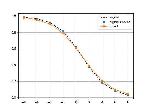
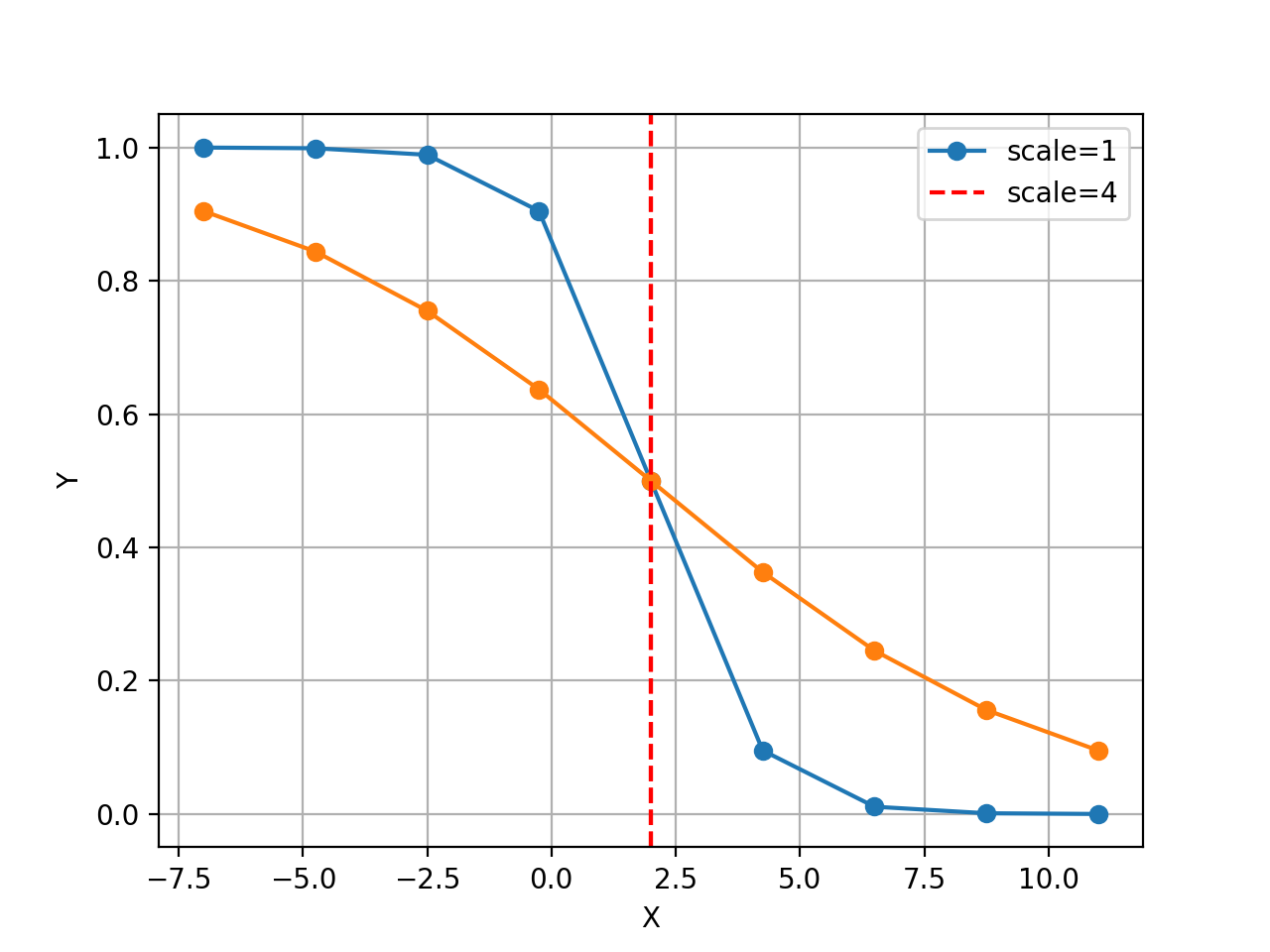
Logistic(xmid, scale, Asym=1, N=9, increase=False)[source]¶ Simple logistic class to see the curve implied by xmid/scale parameters
from gdsctools.logistics import Logistic
from pylab import legend
tl = Logistic(2, 1)
tl.plot()
tl.scale = 4
tl.plot(hold=True)
legend(['scale=1', 'scale=4'])
(Source code, png, hires.png, pdf)
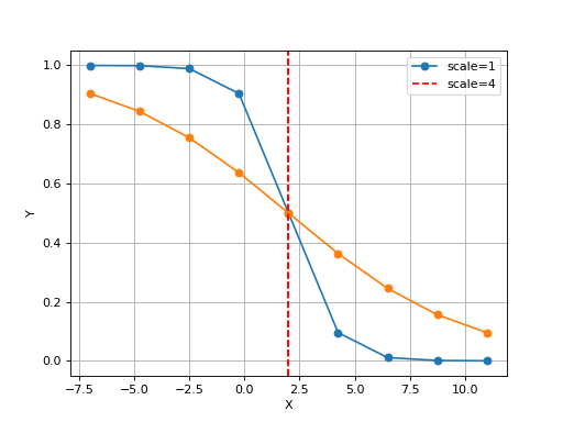
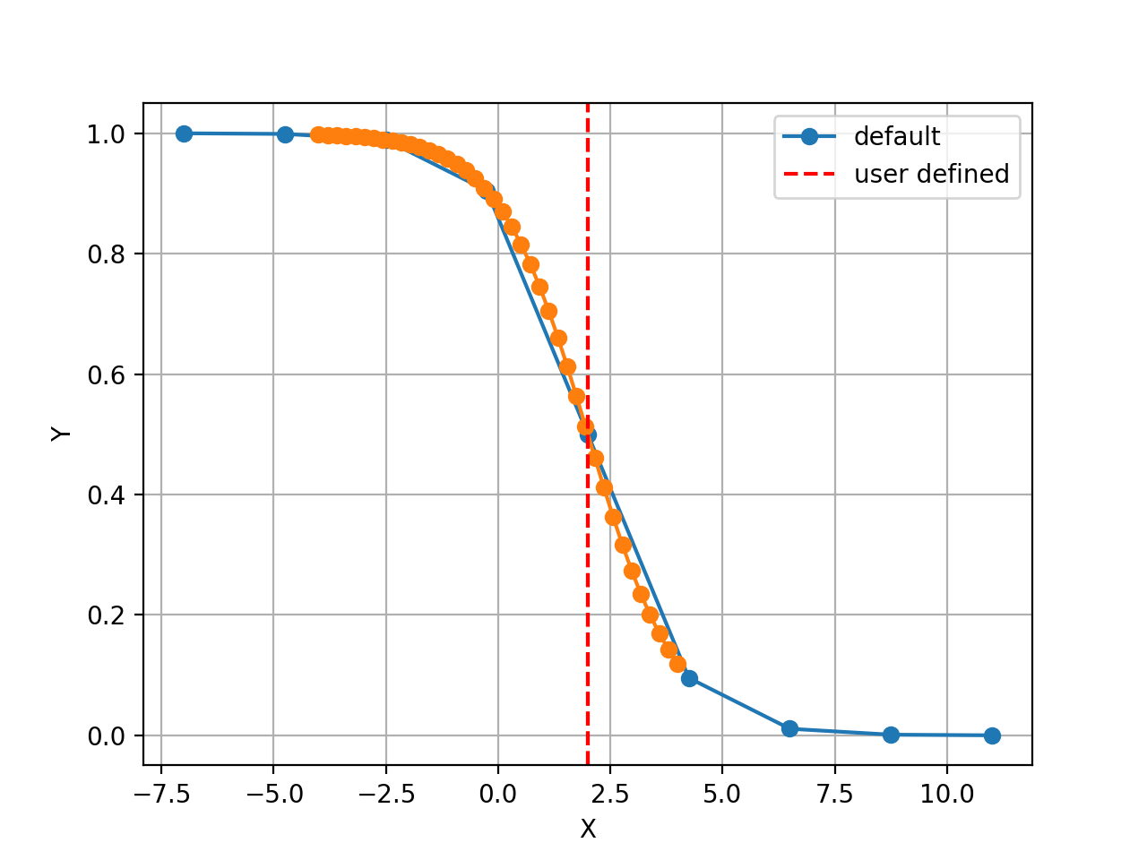
The X values are set automatically given the number of data points
Nand the minimum and maximum X values. By default a sensible values for the minimun and maximum x values are guessed based onscaleparameter but one can set thexminandxmaxfrom gdsctools.logistics import Logistic from pylab import legend tl = Logistic(2,1) tl.plot() tl.xmin= -4 tl.xmax = 4 tl.N = 40 tl.plot(hold=True) legend(['default', 'user defined'])
(Source code, png, hires.png, pdf)

Constructor
Parameters: - xmid – the first logistic function parameter
- scale – the second logistic function parameter
- Asym – Amplitude of the function
- N – number of data point
- increase – increasing or decreasing function.
- xmin – starting range of x-values
- xmax – ending range of x-values
if
increaseis False: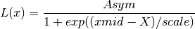
if
increaseis True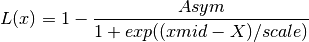
Changing
xmin,xmaxorNdoes change the content of X. You can changeXdirectly.-
N¶ set/get the number points
-
X¶ get/set of the x-values
-
Y¶ Getter for Y-values
-
scale
-
xmax¶ set/get the maximum x range
-
xmin¶ set/get the minimum x range
-
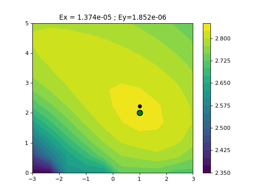
class
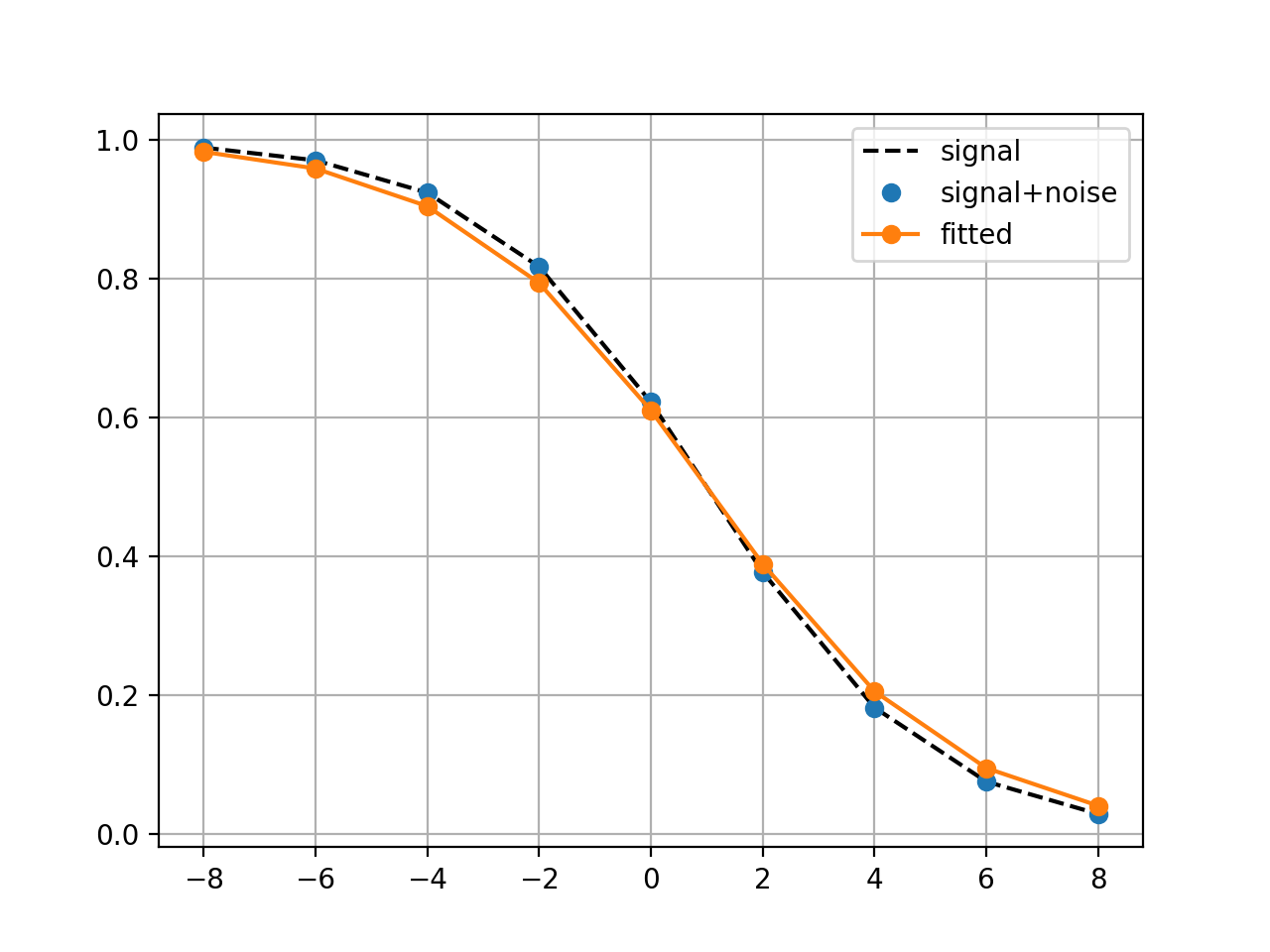
LogisticMatchedFiltering(xmid, scale, N=9)[source]¶ Experimental class to identify parameters of a noisy Logistic function
This class implements two methods to identify the parameters (xmid and scale) of a logistic function.
Note One constraint is to define the x-values.
from gdsctools import logistics
import pylab

mf = logistics.LogisticMatchedFiltering(1,2)
mf.scan(pylab.linspace(-3,3, 10), pylab.linspace(0,5,10))
constructor
Parameters: - xmid –
- scale –
- N –
-
N
-
X¶ get/set the X values the logistic signal
-
scale¶ get/set the scale value of the logistic signal
-
xmid¶ get/set the xmid value of the logistic signal
14.8. Regression Analysis
14.8.1. Common Regression class
-
class
Regression(ic50, genomic_features=None, verbose=False)[source]¶ Base class for all Regression analysis
In the
gdsctools.anova.ANOVAcase, the regression is based on the OLS method and is computed for a given drug and a given feature (ODOF). Then, the analysis is repeated across all features for a given drug (ODAF) and finally extended to all drugs (ADAF). So, there is one test for each combination of drug and feature.Here, all features for a given drug are taken together to perform a Regression analysis (ODAF). The regression algorithm implemented so far are:
- Ridge
- Lasso
- ElasticNet
- LassoLars
Based on tools from the scikit-learn library.
Constructor
Parameters: - ic50 – an IC50 file
- genomic_features – a genomic feature file
see Data Format and Readers for help on the input data formats.
-
boxplot(drug_name, model, n=5, minimum_match_per_combo=10, bx_vert=True, bx_alpha=0.5, verbose=False, max_label_length=40)[source]¶ Boxplot plot of the most important features.
Parameters: # assuming there is a drug ID = 29 r = GDSCLasso() model = r.get_best_model(29) r.boxplot(29, model)
In addition, we also show the wild type case where the total number of mutations is 0.
-
check_randomness(drug_name, kfolds=10, N=10, progress=False, nbins=40, show=True, **kargs)[source]¶ Compute Bayes factor between NULL model and best model fitted N times
Parameters: - drug_name –
- kfolds –
- N (int) – optimise NULL models and real model N times
- progress –
- nbins –
- show –
Bayes factor:
S = sum([s>r for s,r in zip(scores, random_scores)])
proba = S / len(scores)
bayes_factor = 1. / (1-proba)
Interpretation for values of the Bayes factor according to Kass and Raftery (1995).
Interpretation B(1,2) Very strong support for 1 < 0.0067 Strong support 1 0.0067 to 0.05 Positive support for 1 0.05 to .33 Weak support for 1 0.33 to 1 No support for either model 1 Weak support for 2 1 to 3 Positive support for 2 3 to 20 Strong support for 2 20 to 150 Very strong support for 2 > 150
-
dendogram_coefficients(stacked=False, show=True, cmap='terrain')[source]¶ shows the coefficient of each optimised model for each drug
This works for demonstration and small data sets.
-
fit(drug_name, alpha=1, l1_ratio=0.5, kfolds=10, show=True, tol=0.001, normalize=False, shuffle=False, perturbation=0.01, randomize_Y=False)[source]¶ Run Elastic Net with a cross validation for one value of alpha
Parameters: - drug_name – the drug to analyse
- alpha (float) – note that theis alpha parameter corresponds to the lambda parameter in glmnet R package.
- l1_ratio (float) – This is the lasso penalty parameter. Note that in scikit-learn, the l1_ratio correspond to the alpha parameter in glmnet R package. l1_ratio set to 0.5 means that there is a weight equivalent for the Lasso and Ridge effects.
- kfolds (int) – defaults to 10
- shuffle – shuffle the indices in the KFold
Returns: kfolds scores for each fold. The score is the pearson correlation.
Note
l1_ratio < 0.01 is not reliable unless sequence of alpha is provided.
Note
alpha = 0 correspond to an OLS analysis
-
get_best_model(drug_name, kfolds=10, alphas=None, l1_ratio=0.5)[source]¶ Return best model fitted using a CV
Parameters: - drug_name –
- kfolds –
- alphas –
- l1_ratio –
-
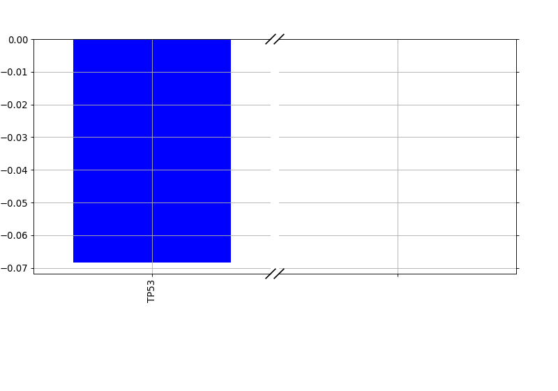
plot_importance(drug_name, model=None, fontsize=11, max_label_length=35, orientation='vertical')[source]¶ Plot the absolute weights found by a fittd model.
Parameters: Returns: the dataframe with the weights (may be empty)
Note
if no weights are different from zeros, no plots are created.
-
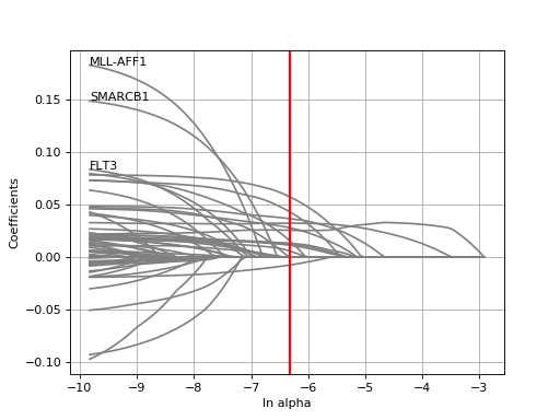
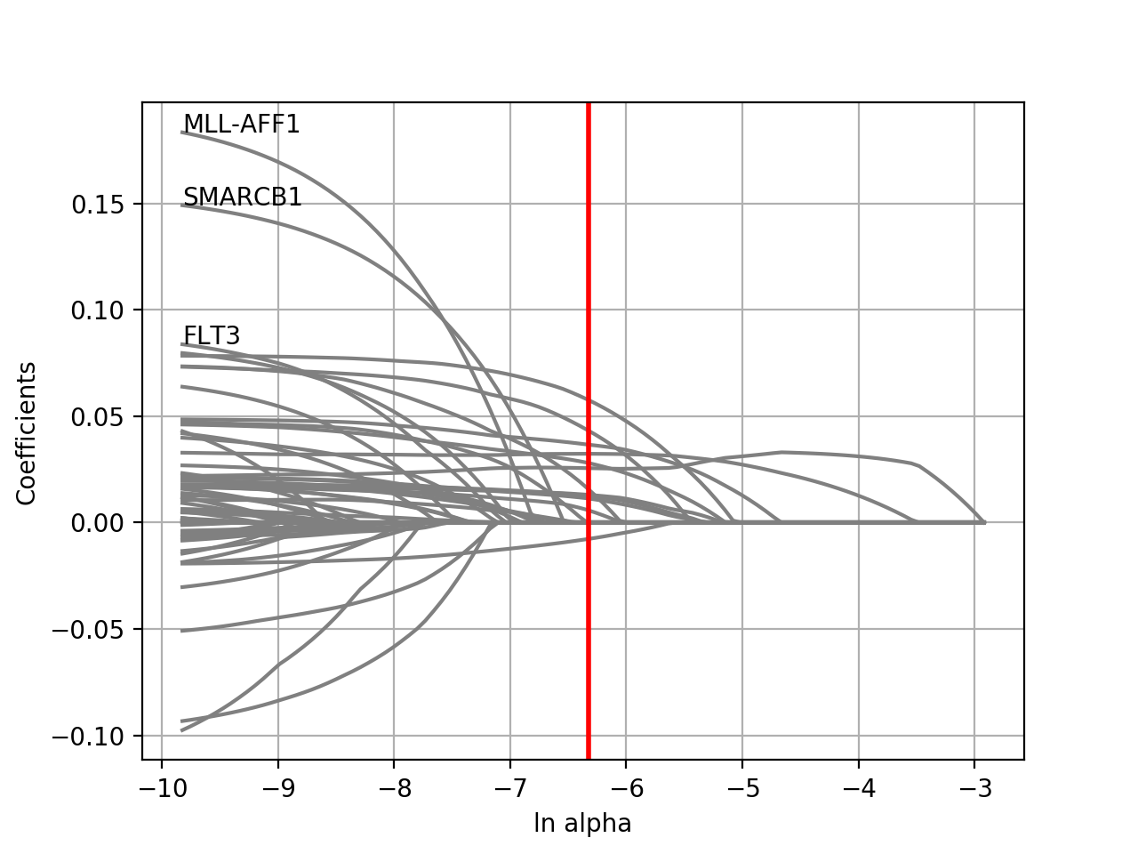
plot_weight(drug_name, model=None, fontsize=12, figsize=(10, 7), max_label_length=20, Nmax=40)[source]¶ Plot the elastic net weights
Parameters: - drug_name – the drug identifier
- alpha –
- l1_ratio –
Large alpha values will have a more stringent effects on the weigths and select only some of them or maybe none. Conversely, setting alphas to zero will keep all weights.
from gdsctools import *
ic = IC50(gdsctools_data("IC50_v5.csv.gz"))
gf = GenomicFeatures(gdsctools_data("genomic_features_v5.csv.gz"))
en = GDSCElasticNet(ic, gf)
model = en.get_model(alpha=0.01)
en.plot_weight(1047, model=model)
(Source code, png, hires.png, pdf)

-
runCV(drug_name, l1_ratio=0.5, alphas=None, kfolds=10, verbose=True, shuffle=True, randomize_Y=False, **kargs)[source]¶ Perform the Cross validation to get the best alpha parameter.
Returns: an instance of RegressionCVResultsthat contains alpha parameter and Pearson correlation value.
-
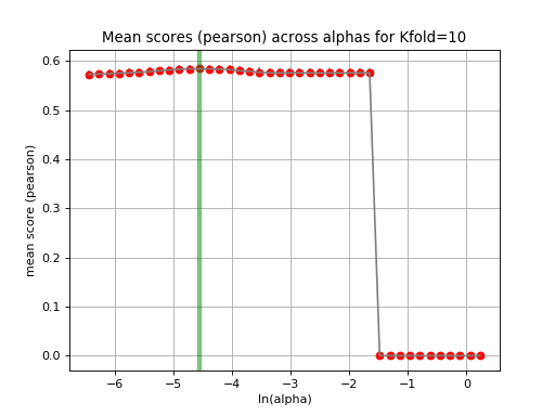
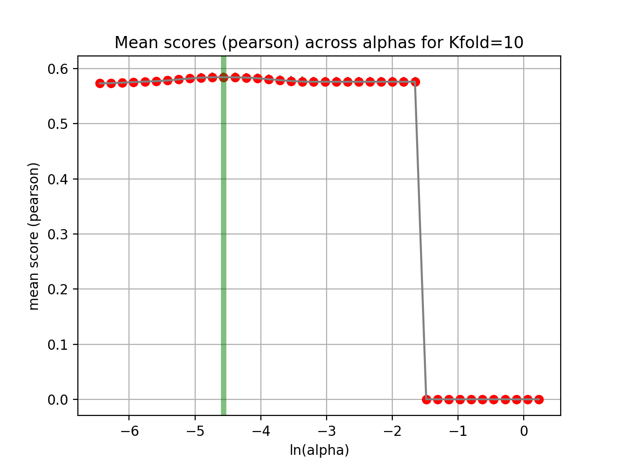
tune_alpha(drug_name, alphas=None, N=80, l1_ratio=0.5, kfolds=10, show=True, shuffle=False, alpha_range=[-2.8, 0.1], randomize_Y=False)[source]¶ Interactive tuning of the model (alpha).
This is much faster than
plot_cindex()but much slower thanrunCV().from gdsctools import * ic = IC50(gdsctools_data("IC50_v5.csv.gz")) gf = GenomicFeatures(gdsctools_data("genomic_features_v5.csv.gz")) en = GDSCElasticNet(ic, gf) en.tune_alpha(1047, N=40, l1_ratio=0.1)
(Source code, png, hires.png, pdf)
14.8.2. Lasso
-
class
GDSCLasso(ic50, genomic_features=None, verbose=False)[source]¶ See as
Regression
14.8.3. ElasticNet
-
class
GDSCElasticNet(ic50, genomic_features=None, verbose=False, set_media_factor=False)[source]¶ Variant of
ANOVAthat handle the association at the drug level using an ElasticNet analysis of the IC50 vs Feature matrices.As compared to the
GDSCRidgeandGDSCLassoHere is an example on how to perform the analysis, which is similar to the ANOVA API:
from gdsctools import GDSCElasticNet, gdsctools_data, IC50, GenomicFeatures
ic50 = IC50(gdsctools_data("IC50_v5.csv.gz"))
gf = GenomicFeatures(gdsctools_data("genomic_features_v5.csv.gz"))

en = GDSCElasticNet(ic50, gf)
en.enetpath_vs_enet(1047)
(Source code, png, hires.png, pdf)
For more information about the input data sets please see
ANOVA,readersConstructor
Parameters: - IC50 (DataFrame) – a dataframe with the IC50. Rows should be the COSMIC identifiers and columns should be the Drug names (or identifiers)
- features – another dataframe with rows as in the IC50 matrix and columns as features. The first 3 columns must be named specifically to hold tissues, MSI (see format).
- verbose – verbosity in “WARNING”, “ERROR”, “DEBUG”, “INFO”
-
enetpath_vs_enet(drug_name, alphas=None, l1_ratio=0.5, nfeat=5, max_iter=1000, tol=0.0001, selection='cyclic', fit_intercept=False)[source]¶ #if X is not scaled, the enetpath and ElasticNet will give slightly # different results #if X is scale using:
from sklearn import preprocessing
xscaled = preprocessing.scale(X)
xscaled = pd.DataFrame(xscaled, columns=X.columns)
-
plot_cindex(drug_name, alphas, l1_ratio=0.5, kfolds=10, hold=False)[source]¶ Tune alpha parameter using concordance index
This is longish and performs the following task. For a set of alpha (list), run the elastic net analysis for a given l1_ratio with kfolds. For each alpha, get the CIndex and find the CINdex for which the errors are minimum.
Warning
this is a bit longish (300 seconds for 10 folds and 80 alphas) on GDSCv5 data set.
14.8.4. Ridge
-
class
GDSCRidge(ic50, genomic_features=None, verbose=False)[source]¶ Same as
Regression
14.8.5. Report
Code related to the Regression analysis to find associations between drug IC50s and genomic features
-
class
RegressionReport(method, directory='.', verbose=True, image_dir='images', data_dir='data', config={'boxplot_n': '?'})[source]¶ Class used to interpret the results and create final HTML report
Constructor
Parameters: - method – Method used in the regression analysis (lasso, elasticnet, ridge)
- results –
14.9. Data Packages
-
class
IC50Cluster(ic50, ratio_threshold=10, verbose=True, cluster=True)[source]¶ Utility to cluster columns that correspond to the same drug ID
From GDSC v18 data sets onwards, DRUG identifiers may be duplicated to account for different drug concentration. This is not recommended since we’d rather use unique identifier for different experiments but to account for this feature, the IC50Cluster will rename the columns and transform the data as follows.
Consider the case of the DRUG 1211. It appears 3 times in the original data:
Drug_1211_0.15625_IC50
Drug_1211_1_IC50
Drug_1211_10_IC50
Actually, there are about 15 such cases even though in general there are only 2 duplicates:
    DRUG_ID   1   2    3  total  icommon       ratio
21     1782  47  47  NaN     47      47  100.000000
20     1510  45  45  NaN     45      45  100.000000
19     1211  48  47  4.0     50      46   92.000000
18     1208  48  47  NaN     50      45   90.000000
16     1032  43  47  NaN     50      40   80.000000
17     1207  38  47  NaN     50      35   70.000000
13      231   2  39  NaN     39       2    5.128205
14      232  45   2  NaN     45       2    4.444444
10      226   2  45  NaN     45       2    4.444444
12      230   2  46  NaN     46       2    4.347826
15      238   2  46  NaN     46       2    4.347826
0       206   2  46  NaN     46       2    4.347826
1       211  46   2  NaN     46       2    4.347826
9       224   2  46  NaN     46       2    4.347826
8       223   2  46  NaN     46       2    4.347826
7       221   2  46  NaN     46       2    4.347826
6       217   2  46  NaN     46       2    4.347826
5       216   2  46  NaN     46       2    4.347826
4       215   2  46  NaN     46       2    4.347826
3       214   2  46  NaN     46       2    4.347826
2       213   2  46  NaN     46       2    4.347826
11      229   2  46  NaN     46       2    4.347826
The clustering works as follows. If the ratio of drugs in common between several concentrations is large, then they are studied independently. Otherwise they are merged.
In the final dataframe, the columns names are transformed into unique identifiers like in the IC50 class by removing the
Drug_prefix and``_conc_IC50suffix.The
mappingcontains the mapping between new and old identifiers.See also
cleanup()method.constructor
Parameters: -
cleanup(offset=10000)[source]¶ Rename the columns into unique identifiers
Parameters: offset (int) – if duplicated, add the offset The
mappingcontains the mapping, which should be used to update the decoder file.
-
duplicated
-
to_cluster
-
-
class
GDSC(ic50, drug_decode, genomic_feature_pattern='GF_*csv', main_directory='tissue_packages', verbose=True)[source]¶ Wrapper of the
ANOVAclass and reports to analyse all TCGA Tissues and companies automatically while creating summary HTML pages.First, one need to provide an unique IC50 file. Second, the DrugDecode file (see
DrugDecode) must be provided with the DRUG identifiers and their corresponding names. Third, a set of genomic feature files must be provided for each TCGA tissue.You then create a GDSC instance:
from gdsctools import GDSC
gg = GDSC('IC50_v18.csv', 'DRUG_DECODE.txt',
    genomic_feature_pattern='GF*csv')
At that stage you may want to change the settings, e.g:
gg.settings.FDR_threshold = 20
Then run the analysis:
gg.analysis()
This will launch an ANOVA analysis for each TCGA tissue + PANCAN case if provided. This will also create a data package for each tissue. The data packages are stored in ./tissue_packages directory.
Since all private and public drugs are stored together, the next step is to create data packages for each company:
gg.create_data_packages_for_companies()
you may select a specific one if you wish:
gg.create_data_packages_for_companies(['AZ'])
Finally, create some summary pages:
gg.create_summary_pages()
You entry point is an HTML file called index.html
Constructor
Parameters: - ic50 – an
IC50file. - drug_decode – an
DrugDecodefile. - genomic_feature_pattern – a glob to a set of
GenomicFeaturefiles.
-
analyse(multicore=None)[source]¶ Launch ANOVA analysis and creating data package for each tissue.
Parameters: - onweb (bool) – By default, reports are created but HTML pages not shown. Set to True if you wish to open the HTML pages.
- multicore – number of cpu to use (1 by default)
-
companies
-
create_data_packages_for_companies(companies=None)[source]¶ Creates a data package for each company found in the DrugDecode file
-
create_summary_pages()[source]¶ Create summary pages
Once the main analyis is done (
analyse()), and the company packages have been created (create_data_packages_for_companies()), you can run this method that will creade a summary HTML page (index.html) for the tissue, and a similar summary HTML page for the tissues of each company. Finally, an HTML summary page for the companies is also created.The final tree direcorty looks like:
|-- index.html
|-- company_packages
|   |-- index.html
|   |-- Company1
|   |   |-- Tissue1
|   |   |-- Tissue2
|   |   |-- index.html
|   |-- Company2
|   |   |-- Tissue1
|   |   |-- Tissue2
|   |   |-- index.html
|-- tissue_packages
|   |-- index.html
|   |-- Tissue1
|   |-- Tissue2
-
tcga
- ic50 – an
14.10. MISC
Sets of miscellaneous tools
-
class
Savefig(verbose=False)[source]¶ A simple class to save matploltib figures in the proper place
Note
For developers only
-
directory¶ directory where to save figures
-
Code related to the ANOVA analysis to find associations between drug IC50s and genomic features
-
class
ANOVASettings(**kargs)[source]¶ All settings used in
gdsctools.anova.ANOVAanalysisThis class behaves as a dictionary but values for a given key (setting) can be accessed and changed easily like an attribute:
>>> from gdsctools import ANOVASettings
>>> s = ANOVASettings()
>>> s.FDR_threshold
25
>>> s.FDR_threshold = 20
It is the responsability of the users or developers to check the validity of the settings by calling the
check()method. Note, however, that this method does not perform exhaustive checks.Finally, the method
to_html()creates an HTML table that can be added to an HTML report.Note
for developers a key can be changed or accessed to as if it was an attribute. This prevents some functionalities (such as copy() or property) to be used normaly hence the creation of the
check()method to check validity of the values rather than using properties.Here are the current values available.
Name Default Description include_MSI_factor True Include MSI in the regression feature_factor_threshold 3 Discard association where a genomic feature has less than 3 positives or 3 negatives values (e.g., 0, 1 or 2) MSI_factor_threshold 2 Discard association where a MSI count has less than 2 positives or 2 negatives values (e.g., 0, or 1). analysis_type PANCAN Type of analysis. PANCAN means use all data. Otherwise, you must provide a valid tissue name to be found in the Genomic Feature data set. pvalue_correction_method fdr Type of p-values correction method used. Could be fdr, qvalue or one accepted by MultipleTestingpvalue_correction_level True Apply pvalue correction globally. If False, applied to ‘drug_level’ only. equal_var_ttest True Assume equal variance in the t-test minimum_nonna_ic50 6 Minimum number of IC50 required to perform an analysis for a given drug. fontsize 25 Used in some plots for labels FDR_threshold 25 FDR threshold used in volcano plot and significant hits pvalue_threshold 0.001 Used to select significant hits see ANOVAReportdirectory html_gdsc_anova Directory where images and HTML documents are saved. savefig False Save the figure or not (PNG format) effect_threshold 0 Used in the volcano plot. See VolcanoPlotThere are parameters dedicated to the regression method. Note that only regression_formula is effective right now.
Name Default Description regression_method OLS Regression method amongst OLS. NOT USED YET. regression_alpha 0.01 Fraction of penalty included. If 0, equivalent to OLS. NOT USED YET. regression_L1_wt 0.5 Fraction of the penalty given to L1 penalty term. Must be between 0 and 1. If 0, equivalent to Ridge. If 1 equivalent to Lasso. NOT USED YET. regression_formula auto if auto, use standard regression from GDSCTools (see link_formula) otherwise any valid regression formula can be used. See also
About the settings or gdsctools.readthedocs.org/en/master/settings.html#filtering decrease the number of significant hits.
Small functionalities to retrive chembl/chemspider identifiers based on a drug name
-
class
ChemSpiderSearch(drug_decode)[source]¶ This class uses ChemSpider and ChEMBL to identify drug name
Warning
this is a draft version in dev mode
c = ChemSpiderSearch()
c.search_in_chemspider()
c.search_from_smile_inchembl()
df = c.find_chembl_ids()
It happens that most of public names can be found and almost none of non-public are found. As expected…
If chemspider, chembl and pubchem are empty, search for the drug name in chemspider.
- CHEMSPIDER search:
- if no identifier found, the search if DROPPED if 1 identifier found, we keep going using the SMILE identifier If more than 1 identifier found, this is AMBIGUOUS.
If chembl and pubchem, check with unichem If chembl, check smiles If chembl and chemspider, check smiles ?
SMILES are not unique
Code related to the ANOVA analysis to find associations between drug IC50s and genomic features
-
class
BaseModels(ic50, genomic_features=None, drug_decode=None, verbose=True, set_media_factor=False)[source]¶ A Base class for ANOVA / ElaticNet models
Constructor
Parameters: - IC50 (DataFrame) – a dataframe with the IC50. Rows should be the COSMIC identifiers and columns should be the Drug names (or identifiers)
- features – another dataframe with rows as in the IC50 matrix and columns as features. The first 3 columns must be named specifically to hold tissues, MSI (see format).
- drug_decode – a 3 column CSV file with drug’s name and targets
see
readersfor more information. - verbose – verbosity in “WARNING”, “ERROR”, “DEBUG”, “INFO”
The attribute
settingscontains specific settings related to the analysis or visulation.-
cosmicIds¶ get/set the cosmic identifiers in the IC50 and feature matrices
-
drugIds¶ Get/Set drug identifers
-
feature_names¶ Get/Set feature names
-
set_cancer_type(ctype=None)[source]¶ Select only a set of tissues.
Input IC50 may be PANCAN (several cancer tissues). This function can be used to select a subset of tissues. This function changes the
ic50dataframe and possibly the feature as well if some are not relevant anymore (sum of the column is zero for instance).
-
settings= None¶ an instance of
ANOVASettings